Let’s Build GPT: from scratch, in code, spelled out

2023-11 · notes · zero to hero

Let's build GPT: from scratch, in code, spelled out.

Background

Transformers

The Transformer architecture comes from the landmark paper Attention Is All You Need.

Attention Is All You Need

At the time of the paper, the dominant language translation models were recurrent neural networks (RNN) with an encoder-decoder structure. During inference, the encoder processes each input token sequentially, updating its own hidden state at each time step. Using the final hidden state of the encoder, the “autoregressive” decoder then starts generating output tokens sequentially, taking generated output tokens as additional input, updating its hidden state at each time step.

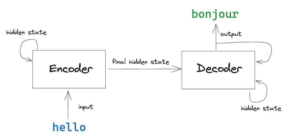
The hidden states of the encoder and decoder gets updated in each time step via a feedback loop that connects the output of each neuron back into itself as an input at the next time step. This feedback loop is what allows recurrent networks and its variants to have “memory” and model long range dependencies in sequences.

A brief introduction to recurrent neural networks (figure lives in the article)

However, the sequential nature of recurrence precludes parallelization “within training examples”. For example, say we are training a RNN with character level tokens. The encoder would need to process each input character sequentially. The autoregressive decoder (even though it takes in “ground truth” tokens instead of generated tokens during training) must also generate predictions for each output character sequentially.

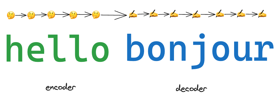
In contrast, the attention mechanism allows the Transformer encoder and decoder to process all input tokens within a training example in parallel. For example, the attention based encoder would be able to process every character in the input sequence AND generate predictions for every single output position in parallel, all in a single forward pass. This ability to parallelize within training examples allowed researchers to scale the Transformer to surpass the previous state of the art performance of recurrent models.

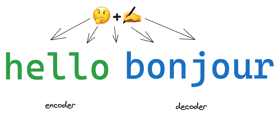
The paper is titled Attention Is All You Need because some of the best performing RNN models at the time also included the attention mechanism. The main point is that the attention mechanism is all you need and that recurrence (along with its scalability problems) can be dispensed with completely.

Architecture

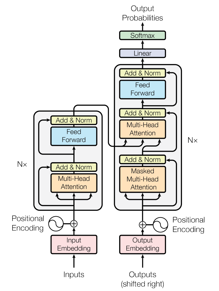
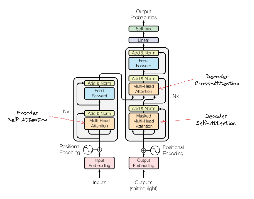
Like the recurrent models, the Transformer also has an encoder (left) and an autoregressive decoder (right). Unlike recurrent models, there is no feedback loop in either the encoder and decoder. Instead, we have Attention layers (in orange) that process the inputs and autoregressive (”shifted right”) outputs in parallel.

Since the model has no knowledge of the sequence order (which is implicit for recurrent networks), the position of each token is encoded and added to the embedding before feeding to the attention layers.

The encoder pays attention to the input via a “multi-head” “self-attention” layer (more on this below). The decoder pays attention to both the autoregressive outputs via a “masked” multi-head self-attention layer (more on this below) and also the inputs via the output of the encoder (also known as “cross-attention”). At each time step, the model is able to “attend to” all inputs and produce probabilities for a single output token.

In both the encoder and decoder, the feed forward layers that comes after the attention layers allows the model to “think” and process the outputs of the attention layers. Together, the attention and feed forward layers form a “block” that is repeated N times.

Attention

At a high level, the attention mechanism is responsible for deciding how much attention to pay to each part of the input sequence. Its output is an attention-weighted representation of the input sequence, which essentially allows consumers of it to “focus” on the most relevant parts.

Q = XW_Q K = XW_K V = XW_V Attention = softmax(QK^T / sqrt(d_k))V

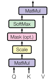
• Query, Key, Value: first we compute 3 sets of vectors for each token in the input: Query (Q), Key (K), and Value (V). These vectors are derived from the input sequence through a linear transformation (with weights W_Q, W_K, and W_V) of the input vector (X) of size (d_k).
  • Query: what information is relevant to each token (d_k)
  • Key: what information is contained in each token (d_k)
  • Value: the information contained in each token (d_k)
• Score: then we compute the score vector by taking the dot product of the Query and Key vectors (QK^T).
  • Score: the relevance of each token to every other token(d_k)
• Scale: scale the scores by 1/sqrt(d_k) to prevent input vectors with large dimensions (d_k) from causing the score to take on large values and pushing the Softmax function below into regions with extremely small gradients.
• (Optional) mask: optionally mask some of the scaled scores to negative infinity, causing the Softmax function below to assign a 0 weight to these positions.
  • Negative infinity score: ignore the interaction between these two tokens
• Weights: apply the Softmax function to turn scaled scores into weights
  • Weights: how much attention to give to each token is based on
• Sum: multiply the attention weights by the Value vector to get the output Attention vector
  • Attention: the weighted sum of all information in the current+preceding tokens

Masked Attention

Recall that the decoder is “autoregressive”. During inference, it consumes its previous output as additional input. During training, it consumes the “ground truth” as additional input instead.

For example, when the decoder is making predictions to generate the 5th token position (where the o is in bonjour), it takes in all previous ground truth characters bonj as additional context.

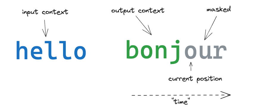
In recurrent models, the fact that each token from the ground truth is fed into the decoder sequentially implicitly “masks” the subsequent tokens, preventing any kind of information leakage from the “future”.

In contrast, the decoder in the Transformer has no real concept of “time” since it generates predictions for every output position in parallel. “Time” is just an internal batch dimension. As a result, we must explicitly “mask” certain tokens from the attention mechanism to prevent information leakage from tokens “from the future” when generating predictions.

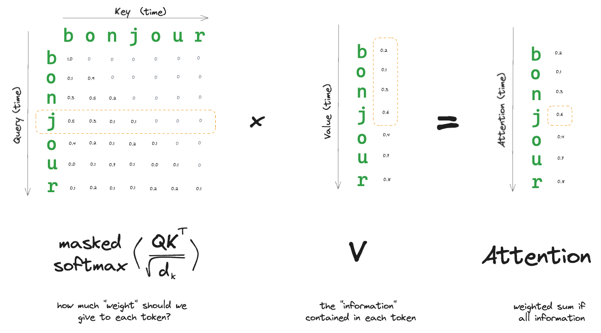
Recall that the attention is the dot product of the attention weights and Value vector. Each value in the Attention output is just the weighted sum of values. If we “mask” the score matrix with -inf for all values in the upper right corner, we will get a weight matrix with 0 for those same positions. This way we essentially prevent information from tokens “in the future” from being included in the weighted sum.

In the diagram below, “information” is a single number, but in practice it would be a vector.

Multi-Head Attention

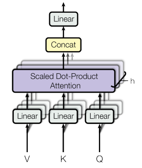
Instead of performing the attention mechanism a single time, the paper proposes to do it multiple times in parallel. Each “head” of attention will get its own set of Q, K, V linear projections. The outputs of each attention head is then concatenated for the final output of the “multi-head” attention.

The reason for multiple heads is to capture different kinds of relationships between tokens. For example, if we are trying to capture relationships between characters, one head might learn to focus the relationship between vowels vs consonants, while another may learn to focus on relationships between alliteration.

Self vs Cross Attention

The terms “self-attention” and “cross-attention” simply refer to whether the attention mechanism is attending to the sequence it is currently processing.

In the encoder, the attention mechanism is processing the input, and attending to tokens in the input, so it is self-attention.

In the decoder, there are 2 attention mechanisms. The one in the bottom of the diagram is processing the autoregressive outputs of the decoder, which is the same sequence that it is processing, so it is also self-attention. But the other attention mechanism that comes afterwards is attending to the output of the encoder, which is a different sequence than the one it is processing, so it is called cross-attention.

Implementation

Architecture

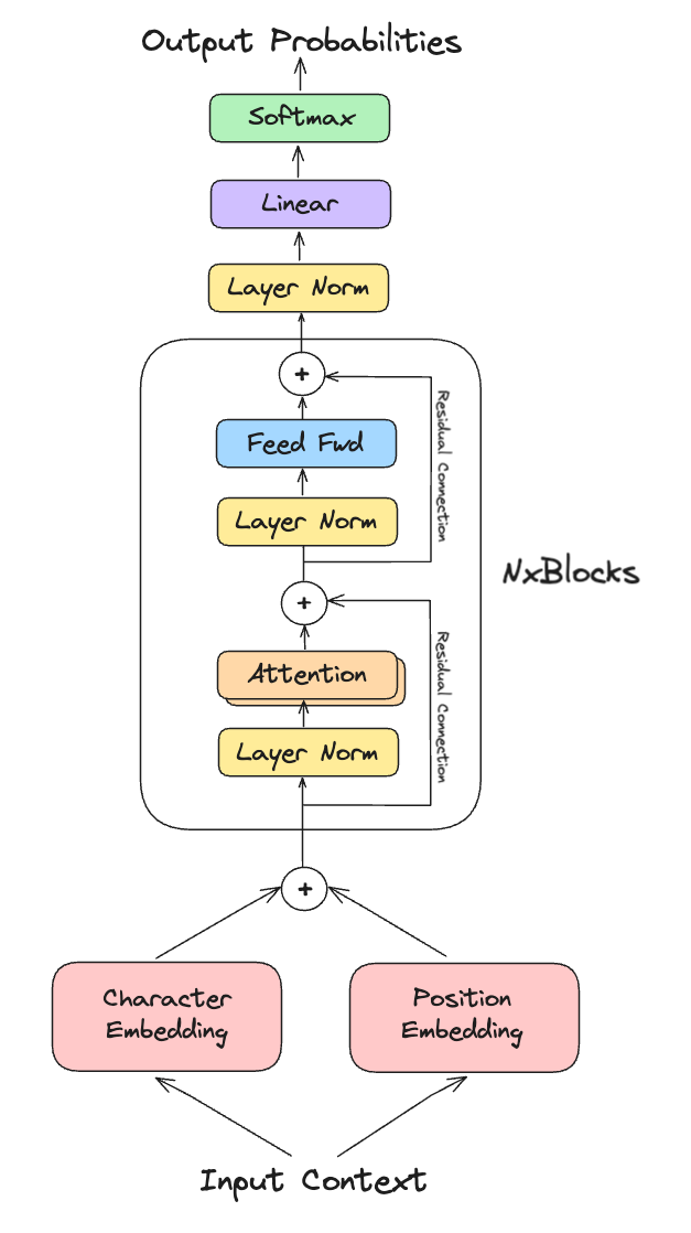
Since the original paper was tackling the problem of machine translation, there is both an encoder and the decoder. Our task is just text generation, so we will only implement the decoder with no encoder and no cross-attention layer.

Another difference is that we normalize before (instead of after) the attention and feed forward layers as this is now common practice.

Lastly, the paper uses a sinusoidal positional encoding but we will just use a simple embedding.

Code

Here is the code for the attention mechanism.

class Head(nn.Module):
    """one head of self-attention"""

    def __init__(self, head_size):
        super().__init__()
        self.key = nn.Linear(n_embd, head_size, bias=False)
        self.query = nn.Linear(n_embd, head_size, bias=False)
        self.value = nn.Linear(n_embd, head_size, bias=False)
        self.register_buffer('tril', torch.tril(torch.ones(block_size, block_size)))
        self.dropout = nn.Dropout(dropout)

    def forward(self, x):
        B,T,C = x.shape
        k = self.key(x) # (B,T,C)
        q = self.query(x) # (B,T,C)

        # compute attention scores ("affinities")
        wei = q @ k.transpose(-2,-1) * C**-0.5 # (B,T,C) @ (B,C,T) = (B,T,T)
        wei = wei.masked_fill(self.tril[:T, :T] ==0, float('-inf')) # (B, T, T)
        wei = F.softmax(wei, dim=-1) # (B, T, T)
        wei = self.dropout(wei)

        # perform the weighted aggregation of the values
        v = self.value(x) # (B, T, C)
        out = wei @ v # (B, T, T) @ (B, T, C) -> (B, T, C)
        return out

class MultiHeadAttention(nn.Module):
    """multiple heads of self-attention in paralell"""
    def __init__(self, num_heads, head_size):
        super().__init__()
        self.heads = nn.ModuleList([Head(head_size) for _ in range(num_heads)])
        self.proj = nn.Linear(n_embd, n_embd)
        self.dropout = nn.Dropout(dropout)

    def forward(self, x):
        out = torch.cat([head(x) for head in self.heads], dim=-1)
        out = self.dropout(self.proj(out))
        return out

Here is the code for the repeating block.

class FeedForward(nn.Module):
    """a simple layer followed by a non-linearity"""
    def __init__(self, n_embd):
        super().__init__()
        self.net = nn.Sequential(
            nn.Linear(n_embd, 4*n_embd),
            nn.ReLU(),
            nn.Linear(4*n_embd, n_embd),
            nn.Dropout(dropout)
        )

    def forward(self, x):
        return self.net(x)

class Block(nn.Module):
    """Transformer block: communication followed by computation"""
    def __init__(self, n_embd, n_head):
        super().__init__()
        head_size = n_embd // n_head
        self.sa_heads = MultiHeadAttention(n_head, head_size)
        self.ffwd = FeedForward(n_embd)
        self.ln1 = nn.LayerNorm(n_embd)
        self.ln2 = nn.LayerNorm(n_embd)

    def forward(self, x):
        x = x + self.sa_heads(self.ln1(x))
        x = x + self.ffwd(self.ln2(x))
        return x

Here is the code for the transformer decoder.

class Model(nn.Module):
    def __init__(self, ):
        super().__init__()
        self.token_embedding_table = nn.Embedding(vocab_size, n_embd)
        self.position_embedding_table = nn.Embedding(block_size, n_embd)
        self.blocks = nn.Sequential(*[Block(n_embd, n_head) for _ in range(n_layer)])
        self.ln = nn.LayerNorm(n_embd)
        self.lm_head = nn.Linear(n_embd, vocab_size)


    def forward(self, idx, targets=None):
        B, T = idx.shape

        # idx and targets are both (B,T) tensor of integers
        tok_emb = self.token_embedding_table(idx) # (B, T, C)
        pos_emb = self.position_embedding_table(torch.arange(T, device=device)) # (T, C)
        x = tok_emb + pos_emb # (B, T, C)
        x = self.blocks(x) # (B, T, C)
        x = self.ln(x) # (B, T, C)
        logits = self.lm_head(x) # (B, T, vocab_size)

        if targets is None:
            loss = None
        else:
            B, T, C = logits.shape
            logits = logits.view(B*T, C)
            targets = targets.view(B*T)
            loss = F.cross_entropy(logits, targets)
        return logits, loss

    def generate(self, idx=None, max_new_tokens=1):
        # idx is (B, T) array of indices in the current context
        for _ in range(max_new_tokens):
            B, T = idx.shape
            # crop idx to last block_size tokens
            idx_cond = idx[:, -block_size:] # (B, T)
            # get the predictions
            logits, _loss = self(idx_cond)
            # focus only on the last time step
            logits = logits[:, -1, :] # becomes (B, C)
            # apply softmax to get probabilities
            probs = F.softmax(logits, dim=-1) # (B, C)
            # sample from the distribution
            idx_next = torch.multinomial(probs, num_samples=1) # (B, 1)
            # append sampled index to the running sequence
            idx = torch.cat((idx, idx_next), dim=1) # (B, T+1)
        return idx

Here is the training loop

model = Model()
m = model.to(device)

# create a pytorch optimizer
optimizer = torch.optim.AdamW(model.parameters(), lr=learning_rate)

start = time.time()
for iter in range(max_iters):
    # sample a batch of data
    xb, yb = get_batch('train')

    # evaluate the loss
    logits, loss = model(xb, yb)
    optimizer.zero_grad(set_to_none=True)
    loss.backward()
    optimizer.step()

    # every once in a while evaluate the loss on trai/val
    if iter % eval_interval == 0:
        losses = estimate_loss()
        print(f"step {iter}/{max_iters}: train loss {losses['train']:.4f}, val loss {losses['val']:.4f}")

# print time elapsed
end = time.time()
print(f"total training time {humanize.naturaldelta(end - start)}")

And finally here is how to sample from it

idx = torch.zeros((1, 1), dtype=torch.long)
res = m.generate(idx, max_new_tokens=300)
print(decode(res[0].tolist()))