Makemore Part 1 - Bigram Model

2023-10 · notes · zero to hero

Video: The spelled-out intro to language modeling: building makemore

Problem

How do you create a model of natural language and use it generate text?

Bigram Model

A Bigram Model is a super simple type of language model. The key idea is to use the observed frequencies of one character following another to generate new sequences of characters with a similar distribution.

In this example, we will create a Bigram model using a list of names and try to generate more names.

Bigrams

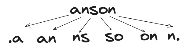
A “bigram” is just a pair of adjacent characters (or syllables or words). For example, the character bigrams of the string anson would just be an, ns, so, and on. If we also consider the start and end of words as special characters ., then we end up with 2 additional bigrams .a and n.

# break "Anson" into bigrams
w = 'anson'
chs = ['.'] + list(w) + ['.']
bigrams = zip(chs, chs[1:])
list(bigrams)
# --> [('.', 'a'), ('a', 'n'), ('n', 's'), ('s', 'o'), ('o', 'n'), ('n', '.')]

Frequency Matrix

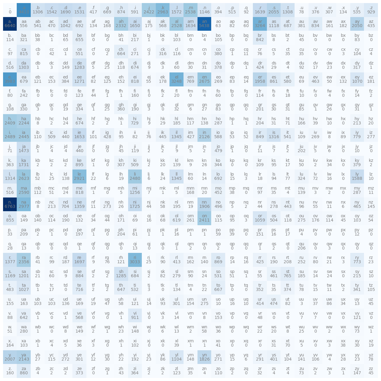
Given a list of names, we can deconstruct each name into its bigrams, and store the frequencies of each unique bigram into a table.

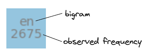
• Each cell in the table contains the bigram and its observed frequency. The darker the background the higher the frequency.
• Cells within the same row contain bigrams that start with the same character. For example, the first row contain all bigrams starting with ..

# Initialize empty matrix
N = torch.zeros((27, 27), dtype=torch.int32)

# Create helper mappings between characters and positional indices
chars = sorted(list(set(''.join(words))))
stoi = {ch: i+1 for i, ch in enumerate(chars)}
stoi['.'] = 0
itos = {i: ch for ch, i in stoi.items()}

# Count frequencies
for w in words:
    chs = ['.'] + list(w) + ['.']
    for ch1, ch2 in zip(chs, chs[1:]):
        N[stoi[ch1], stoi[ch2]] += 1

Probability Matrix

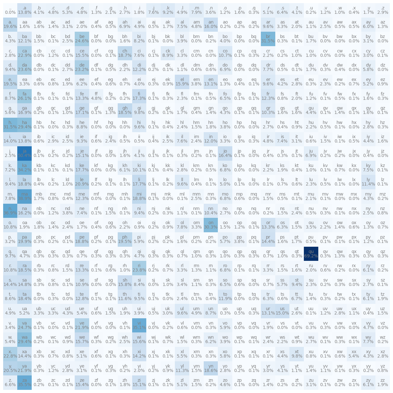
If we normalize each row into probabilities, we will have a lookup table that allows us to easily look up the probabilities of the next character given the current character.

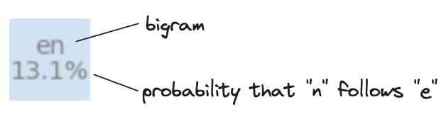
• Each cell in the table contains the bigram and the probability that the second character in the bigram follows the first.
• Since cells within the same row contain bigrams that start with the same character, the sum of probabilities within a row is exactly 1.

# Add a bit of smoothing to prevent 0 probabilities
P = (N+1).float()
# normalize counts N into probabilities P (with smoothing)
P /= P.sum(dim=1, keepdim=True)

Note that we added a “fake count” of 1 to each cell to prevent any cell from having exactly 0 probability which will cause us to have infinite loss below which is ugly and also potentially undesirable since our model will never be able to generate any bigrams it has never seen before. We call this “smoothing”, and the more fake counts we add, the more uniform the probability distributions will become.

Name generation

To generate a new name, all we have to do is to

1. start with the . character
2. randomly pick the next character based on the distribution of probabilities
3. repeat the process until you get the . character again

# generate 10 samples
for i in range(10):
    # start with `.`
		ix = 0
    print(itos[ix], end='')
    while True:
        # pick out the row of probabilities corresponding to the current character
				p = P[ix]
				# randomly pick the next character by sampling the row of probabilities
        ix = torch.multinomial(p, num_samples=1, replacement=True, generator=g).item()
        print(itos[ix], end='')
				# repeat until we get `.` again
				if ix == 0:
            print()
            break

Loss

How do we measure the quality of our model? It is conventional in ML to measure quality of models in terms of “loss”, where loss=0 is considered the perfect score.

There are many different “loss functions”. In this example, we will use the “negative log likelihood” or NLL loss function.

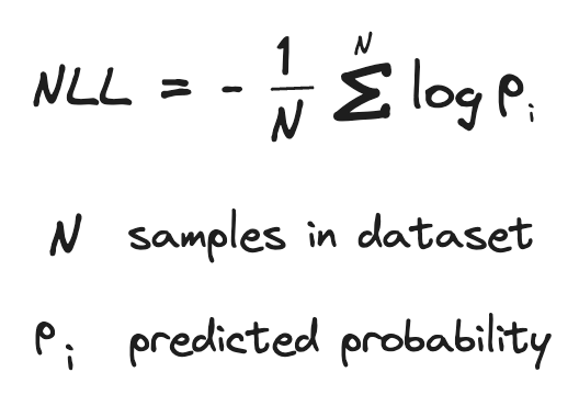
For example, to compute our model’s NLL over our list of names, we can simply break down each name into N bigrams, sum up the log probabilities of the 2nd character following the 1st character (P_i), then negate and divide by N.

log_likelihood = 0 # running sum of log probabilities
n = 0 # number of samples

# for every word in the dataset
for w in words:

    # break down into bigrams
    chs = ['.'] + list(w) + ['.']
    bigrams = zip(chs, chs[1:])

    # for every bigram
    for ch1, ch2 in bigrams:
        # lookup probability of ch2 given ch1
        ix1 = stoi[ch1]
        ix2 = stoi[ch2]
        prob = P[ix1, ix2]

        # add log likelihood to running sum
        logprob = torch.log(prob)
        log_likelihood += logprob

        # increment number of samples
        n += 1

# compute loss
loss = -log_likelihood / n
print(f'loss: {loss:.4f}')

PyTorch Version

Instead of building our bigram model with raw Python dictionaries and counting frequencies by hand, lets use PyTorch to train one (a mathematically identical model).

At a high level, we will construct a weight matrix W that is sort of similar to the count matrix N above. But instead of counting bigrams, we will use gradient descent to learn the weights in W. And instead of going through each sample in a for loop, we can vectorize our calculations for performance.

import torch.nn.functional as F

# create the training set of the bigrams
xs, ys = [], []
for w in words:
    chs = ['.'] + list(w) + ['.']
    for ch1, ch2 in zip(chs, chs[1:]):
        xs.append(stoi[ch1])
        ys.append(stoi[ch2])
xs = torch.tensor(xs) # every 1st character in bigrams
ys = torch.tensor(ys) # every 2nd character in bigrams

# Initialize random weights
W = torch.randn((27, 27), generator=g, requires_grad=True)

# Learn weights with gradient descent
for k in range(100):
    # <--- forward pass --->
		# "pluck out" rows of weights for each x as logits (same as log counts)
    xenc = F.one_hot(xs, num_classes=27).float()
		logits = xenc @ W
		# exponentiate to get counts (equivalent to row in N matrix above)
    counts = logits.exp()
		# normalize to produce probabilities
    probs = counts / counts.sum(dim=1, keepdim=True)
		# compute NNL loss across
    loss = -probs[torch.arange(len(ys)), ys].log().mean()
		# add regularization
		loss += 0.01*(W**2).mean()

    # <--- backward pass --->
    W.grad = None # zero out the gradients
    loss.backward() # compute the gradients
    W.data -= 50 * W.grad # update the weights

Plucking out weights with one hot encoding and matrix multiplication

# "pluck out" rows of weights for each x as logits (same as log counts)
xenc = F.one_hot(xs, num_classes=27).float()
logits = xenc @ W

In the code above, we are using one hot encoding and matrix multiplication to “pluck out” the desired row of weights from W. How does this work?

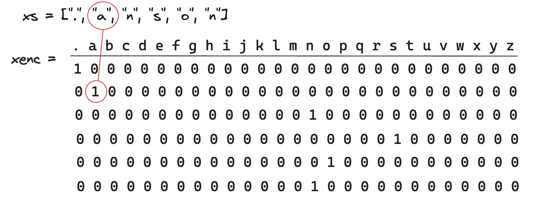
Recall that xs is just the list of every 1st character (index) and ys is the list of every 2nd character (index) in our dataset. For example if our dataset only contains one name anson, then xs would be the indices corresponding to [., a, n, s, o, n] and ys would be indices corresponding to [a, n, s, o, n, .], and N=6.

One hot encoding is a technique used to transform categorical labels into binary vectors. In our case, we are encoding each character label into a binary vector in character space, where we have 27 characters. For example, the character a would have a 1 in the a column and 0 for all other columns. In this way, the list of characters xs with length N would be transformed into a list of binary vectors xenc with shape Nx27.

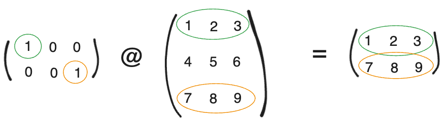
To illustrate how xenc @ w is the same as “plucking out” the rows from W corresponding to each character in xs, let us just consider the following toy example.

Logits and Probabilities

# exponentiate to get counts (equivalent to row in N matrix above)
counts = logits.exp()
# normalize to produce probabilities
probs = counts / counts.sum(dim=1, keepdim=True)

“Logits” refer to the raw, unnormalized values generated by a neural network before being transformed into probabilities.

In our case, logits is a Nx27 matrix, where each row is plucked from W for each x in xs. We interpret each of these numbers as “log counts”. We exponentiate each value to get counts, then we normalize per row to get probs, a Nx27 matrix where each row corresponds to the probability distribution of next characters for each character x in xs.

Vectorized Loss

# compute NNL loss across
loss = -probs[torch.arange(len(ys)), ys].log().mean()
# add regularization
loss += 0.01*(W**2).mean()

We compute the NNL loss in the same way as we did before except again in vectorized form.

If we wanted to get the ith row jth column out of probs, we could do probs[i, j]. If we wanted to get multiple such values, we can instead do probs[is, js] where is is the list of all row indexes i and js is the list of all column indexes js.

Since torch.arange(len(ys)) is just the enumeration of each sample index, and ys is the list of all next characters, probs[torch.arange(len(ys)), ys] will give us the probability of all next characters for each sample.

We then take the log of each value, and then mean across all values, and finally negate to get the NLL.

Regularization

# add regularization
loss += 0.01*(W**2).mean()

Recall that we added a bit of smoothing to our probability matrix above in our non-PyTorch implementation. The more fake counts we add, the smoother or more uniform the probability distribution will become.

In our PyTorch implementation, we achieve the same thing by adding a penalty term to our loss function. If all the values of W are 0, then all logits will be 0, and then counts (which is logits.exp()) will be all 1, and the probabilities will be exactly uniform. This means that bringing the values of W closer to 0 is the same as adding more fake counts above.

In particular what we can do is add a regularization term (W**2).mean() to our loss function, which will be 0 only if W is all 0. This means that we will have loss not only if we have NLL, we will also see some loss if W is not 0.

When we do the gradient descent, we will not only try to move values of W around to minimize NLL, we will also be trying to pull values of W closer to 0. The constant 0.01 is the regularization strength, or how much we want the regularization term to impact our loss function.

Name generation

To generate names with our PyTorch implementation, all we need to do is

• Start with the . character
• Pick the next character by
  • One hot encoding the current character
  • Matrix multiply with weights to get logits
  • Exponentiate to get counts
  • Normalize to get probabilities
  • Sample probabilities to pick next character
• Repeat until you get the . character again

for i in range(10):
    out = []
    ix = 0
    while True:
        xenc = F.one_hot(torch.tensor([ix]), num_classes=27).float()
        logits = xenc @ W
        counts = logits.exp()
        p = counts / counts.sum(1, keepdims=True)
        ix = torch.multinomial(p, num_samples=1, replacement=True, generator=g).item()
        if ix == 0:
            break
        out.append(itos[ix])
    print(''.join(out))