Makemore Part 2 - Multilayer Perceptron

2023-10 · notes · zero to hero

Background

Based on the paper A Neural Probabilistic Language Model by Bengio et al. in 2003.

Problem

N-gram language models are limited by the curse of dimensionality.

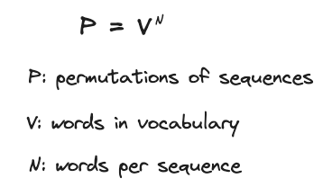
Since the number of permutations of sequences (and thus number of model parameters) scale exponentially with N, it is not practical to scale N even though there is obvious value in considering more context.

At the same time, the high number of sequence permutations makes it is unlikely that sequences in the test set will also be in the training set, which limits the model’s ability to generalize.

Multilayer Perceptron (MLP)

The MLP model solves the curse of dimensionality by projecting high-dimensional word sequences (in discrete space) into a lower-dimensional vector space “embedding”, which captures the semantic relationship between words (in smooth continuous space).

Instead of learning the joint distribution of exact word sequences directly, the MLP model simultaneously learns the embedding and the joint distribution of word sequences expressed by the embedding. With this approach, the number of parameters only scale linearly with V.

Embedding

The sentence “The cat is walking in the bedroom” should help us generalize to make the sentence “A dog was running in a room” because “cat” and “dog” (resp. “is” and “was”, … etc) have similar semantic and grammatical roles.

A hypothetical 3-dimensional embedding of these words might look something like this. Each word is represented by a 3-dimensional vector. Words that are semantically similar would be “close” to each other, and the similarity of two words can be measured by the distance between the two vectors with cosine similarity.

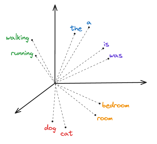
The higher the number of dimensions in the embedding, the deeper the semantic relationship potentially captured.

Network Architecture

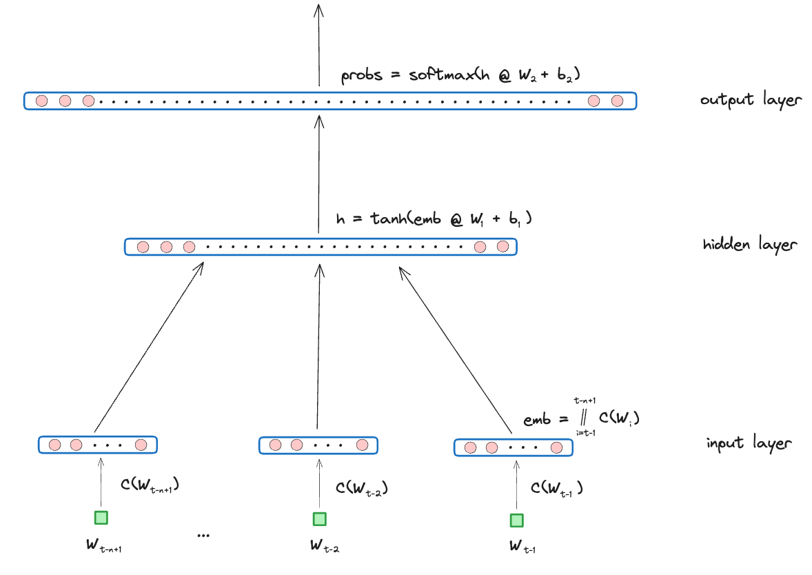
There are 3 layers to the neural network: the input layer, the hidden layer, and the output layer.

First, each of the N previous words in the context are transformed into vectors via a learned embedding lookup table C with D number of dimensions. These embedded vectors are concatenated to form the values of the input layer, so the size of the input layer is simply NxD.

Then, the hidden layer is a linear layer with learned weights W_1 and biases B_1 and a tanh activation function. The size of the hidden layer is a hyper-parameter.

Finally, the output layer is also a linear layer with learned weights W_2, biases B_2 and a softmax activation function. The size of the output layer is V (number of words in the vocabulary).

Implementation

Let’s implement a MLP, but at the character level instead of at the word level. We will be using the same list of names we used in our previous bigram model.

Data

We will split the list of words into train (80%), validation (10%) and test (10%). Each set of words will then be made into blocks of 5 characters, where the first 4 characters will be used as the context, and the 5th character will be used as the target.

import torch
import torch.nn.functional as F

# read in all the words
words = open('names.txt', 'r').read().splitlines()

# build the vocabulary of characters and mappings to/from integers
chars = sorted(list(set(''.join(words))))
stoi = {c:i+1 for i,c in enumerate(chars)}
stoi['.'] = 0
itos = {i:c for c,i in stoi.items()}
print(itos)

# build the train/test/split
block_size = 5
def build_dataset(words):
    X, Y = [], []
    for w in words:
        context = [0] * block_size
        for ch in w + '.':
            ix = stoi[ch]
            X.append(context)
            Y.append(ix)
            context = context[1:] + [ix]
    return torch.tensor(X), torch.tensor(Y)

import random
random.seed(42)
random.shuffle(words)
n1 = int(len(words) * 0.8)
n2 = int(len(words) * 0.9)

Xtr, Ytr = build_dataset(words[:n1])
Xdev, Ydev = build_dataset(words[n1:n2])
Xte, Yte = build_dataset(words[n2:])

Training

Below is the code for model initialization and training. Once we understand the background of the MLP model, the actual code to train it is pretty straightforward.

g = torch.Generator().manual_seed(2147483647)

chars = 27 # number of characters in vocabulary
dimensions = 10 # number of dimensions in embedding
neurons = 10 # number of neurons in hidden layer

# initialize parameters with random values
C = torch.randn((chars, dimensions), generator=g)
W1 = torch.randn((dimensions*block_size, neurons), generator=g)
b1 = torch.randn(neurons, generator=g)
W2 = torch.randn((neurons, chars), generator=g)
b2 = torch.randn(chars, generator=g)
params = [C, W1, b1, W2, b2]

# tell PyTorch to track gradients for all parameters
for p in params:
    p.requires_grad_()

stepi = []
losstri = []
training_steps = 200000
for i in range(training_steps):
    # minibatch
    batch_size = 32
    ix = torch.randint(0, Xtr.shape[0], (batch_size,))

    # forward pass on just minibatch
    emb = C[Xtr[ix]]
    h = torch.tanh(emb.view(-1, block_size*dimensions) @ W1 + b1)
    logits = h @ W2 + b2
    loss = F.cross_entropy(logits, Ytr[ix])

    # backward pass
    for p in params:
        p.grad = None
    loss.backward()

    # update parameters
    lr = 0.1 if i < 100000 else 0.01
    for p in params:
        p.data -= lr * p.grad

    # track stats
    stepi.append(i)
    losstri.append(loss.item())

    print(i, loss.item())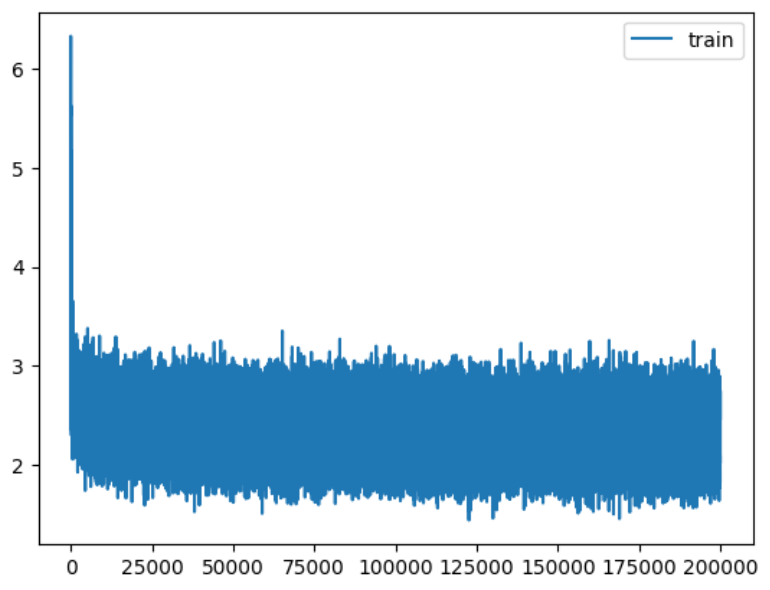

Evaluation

Note that the loss we looked at above was only the loss of each mini batch during the training phase. Here is the actual loss on the train, val, and test splits.

for X, Y in [(Xtr, Ytr), (Xdev, Ydev), (Xte, Yte)]:
    emb = C[X] # embedding lookup (32, 3, 2)
    h = torch.tanh(emb.view(-1, block_size*dimensions) @ W1 + b1) # (32, 100)
    logits = h @ W2 + b2 # (32, 27)
    loss = F.cross_entropy(logits, Y) # (32, 100)
    print(loss.item())

# 2.2879016399383545
# 2.2845089435577393
# 2.2882678508758545

Cross Entropy Loss

We are actually using the same loss function (negative log likelihood) as before. But instead of writing it out we are using PyTorch cross_entropy which is the same thing.

Minibatch

Instead of feeding in the entire dataset of training data to the forward pass on every training loop, we only feed in a randomly sampled “minibatch” of training data.

This makes the training loop much faster.

Learning rate decay

Instead of using a single learning rate throughout the training loop, we decay the learning rate in fixed intervals of steps to help the model “fine tune” itself.

Visualizing the character embedding

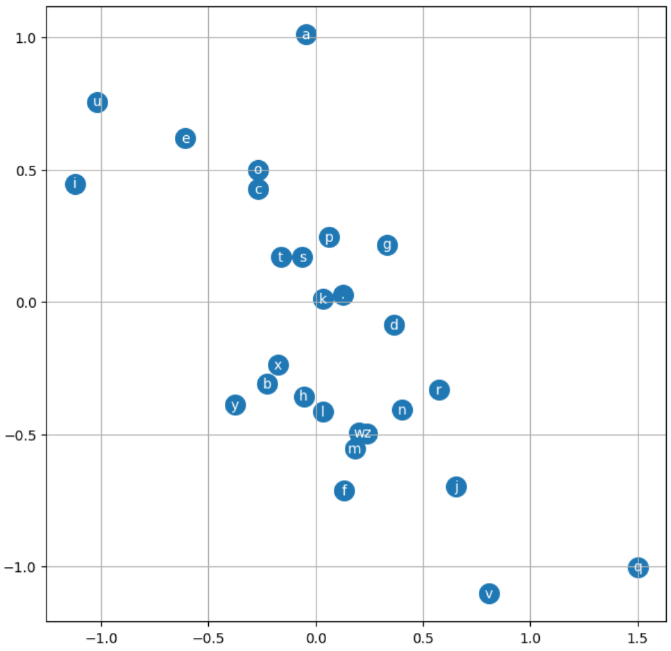
Here is a plot of the first dimension of the embedding. You can sort of see some structure here: the vowels are grouped together in the top left region, all the consonants are in the middle area, and the letters “v” and “q” are far away in the bottom right.

Sampling from the model

Here is the code to sample from the model. We initialize the context with all . characters so the model is free to generate any name.

# sample fom the model
g = torch.Generator().manual_seed(2147483647)
for _ in range(1000):
    out = []
		# initialize context with all `.` characters
    context = [0] * (block_size)
    while True:
        emb = C[torch.tensor([context])]
        h = torch.tanh(emb.view(1, -1) @ W1 + b1)
        logits = h @ W2 + b2
        probs = F.softmax(logits, dim=1)
        ix = torch.multinomial(probs, 1, generator=g).item()
        context = context[1:] + [ix]
        out.append(ix)
        if ix == 0:
            break

    print(''.join([itos[i] for i in out[:-1]]))