Makemore Part 3 - Activations & Gradients, BatchNorm
Improving our basic MLP
This is the MLP we ended up with in the previous lesson.
g = torch.Generator().manual_seed(2147483647)
dimensions = 10
neurons = 200
C = torch.randn((vocab_size, dimensions),           generator=g)
W1 = torch.randn((dimensions*block_size, neurons),  generator=g)
b1 = torch.randn(neurons,                           generator=g)
W2 = torch.randn((neurons, vocab_size),             generator=g)
b2 = torch.randn(vocab_size,                        generator=g)

params = [C, W1, b1, W2, b2]
for p in params:
    p.requires_grad_()

stepi = []
lossi = []
training_steps = 200000

for i in range(training_steps):
    # minibatch
    batch_size = 32
    ix = torch.randint(0, Xtr.shape[0], (batch_size,))

    # forward pass
    emb = C[Xtr[ix]]
    embcat = emb.view(emb.shape[0], -1)
    hpreact = embcat @ W1 + b1
    h = torch.tanh(hpreact)
    logits = h @ W2 + b2
    loss = F.cross_entropy(logits, Ytr[ix])

    # backward pass
    for p in params:
        p.grad = None
    loss.backward()

    # update
    lr = 0.1 if i < (training_steps * 0.5) else 0.01
    for p in params:
        p.data -= lr * p.grad

    stepi.append(i)
    lossi.append(loss.log().item())

    if i % 1000 == 0:
        print(f'{i:6d}/{training_steps:6d}: {loss.item():.4f}')
Fixing the initial loss
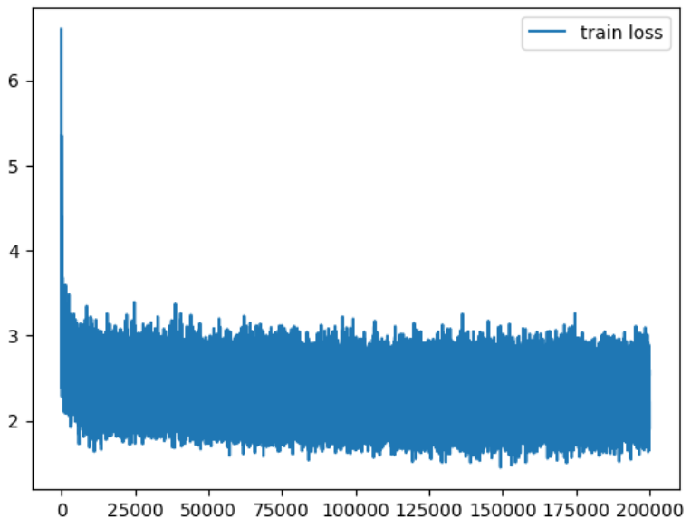
Recall that our training loss chart looked like this, where start with a very high loss and quickly descend in the first few thousand iterations like a hockey stick. The reason why we have this high loss in the beginning is because we initialized our weights with random values. The result is that the logits coming out of the model (right before softmax) are taking on extreme values in the beginning. In a sense, this is like being very “confidently wrong” when in reality we should be much less confident.
What we want instead is for the logits to be more uniform and for symmetry ideally around 0. Recall that logits = h @ W2 + b2. So the simple way we can do this is just to multiply w1 by 0.01 (greatly reduce magnitude) and set b2 to 0 (no bias).
W2 = torch.randn((neurons, vocab_size),             generator=g) * 0.01
b2 = torch.randn(vocab_size,                        generator=g) * 0
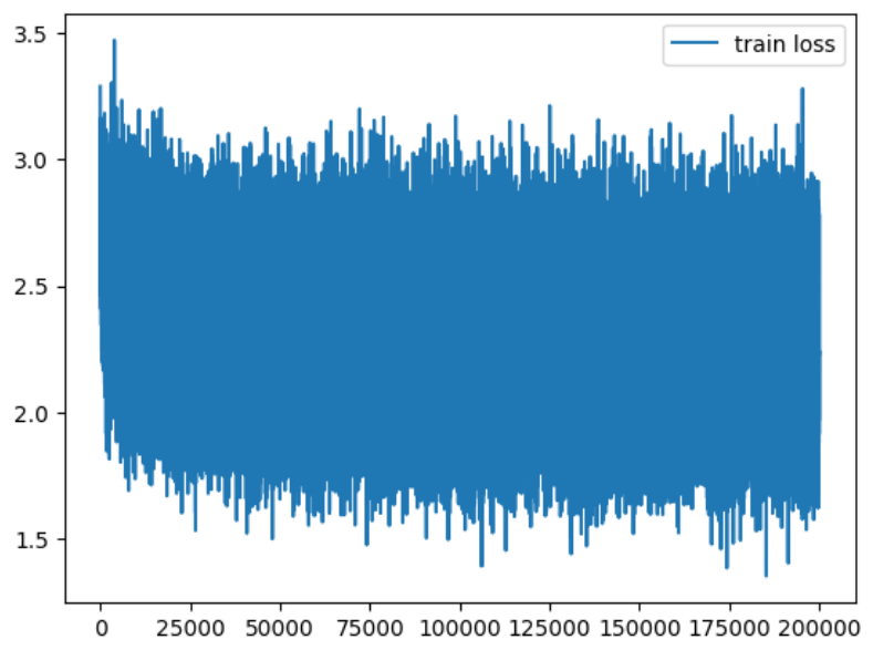
By make this simple change, our train loss no longer exhibits the hockey stick shape in the beginning. This is desirable because the training loop is spending less iterations fixing the overconfidence in the beginning, and more iterations actually learning something useful.
Fixing the initial saturated tanh
If we pause our training loop and visualize the values of h (across all neurons) we can see that the values it takes on is mostly -1 or 1. Recall that h = torch.tanh(hpreact). If we take a look at hpreact, we see that the values have a wide distribution.
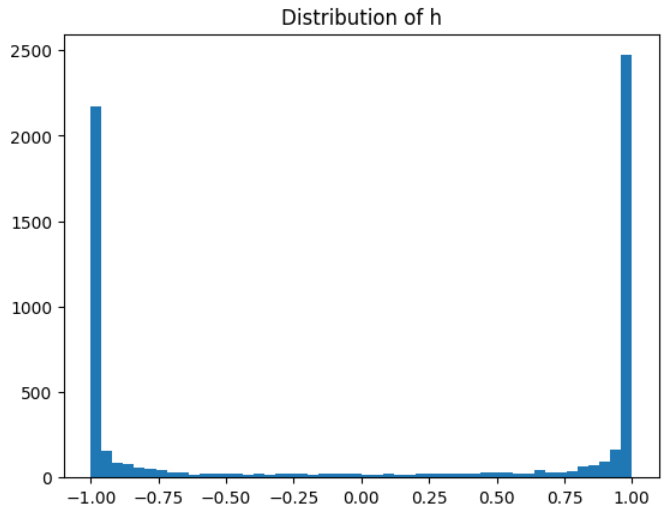
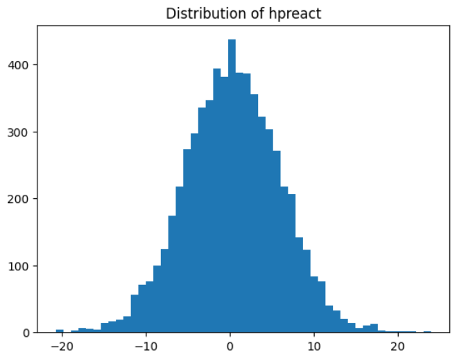
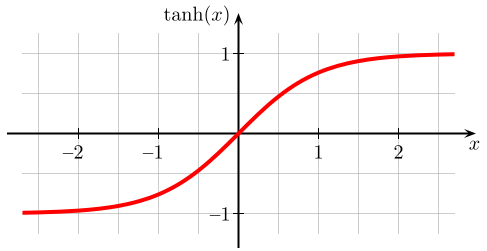
Recall that tanh has this shape. So if the distribution of the inputs are too wide, then you will almost always just be in the flat regions near -1 and 1. This is a problem because the gradient near the flat parts of the tails is very close to 0. This means that backward pass won’t have any impact on it.
If any single neuron only ever takes on the -1 and 1 values, then it is basically a dead neuron and can never learn. One way to visualize this is to check if any neuron has h in the tail regions for all its inputs (a solid white column). Fortunately, we don’t have any dead neurons here. This means that each neuron at least SOME inputs where it is not completely -1 and 1, so it will learn.

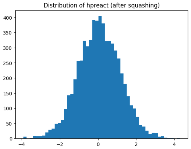
To fix this problem, we just need to squash the distribution of hpreact. Recall that hpreact = embcat @ W1 + b1. The activations now look much better.
W1 = torch.randn((dimensions*block_size, neurons),  generator=g) * 0.2
b1 = torch.randn(neurons,                           generator=g) * 0.01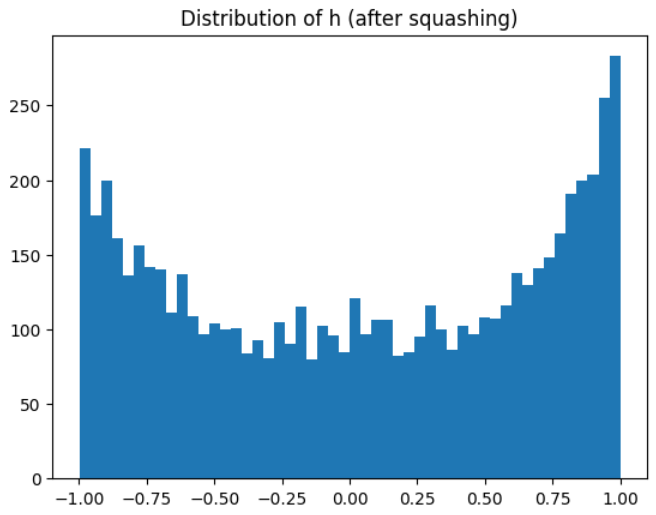

Kaiming initialization
Is there a more principled way to set these multipliers?
We first notice that activations tend to increase in variance as we go forward through the layers. This is because two unit Gaussian distributions (μ=0, σ=1) multiplied together will yield a Gaussian distribution that has higher standard deviation.
x = torch.randn(1000, 10)
w = torch.randn(10, 200)
y = x @ w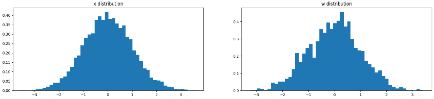
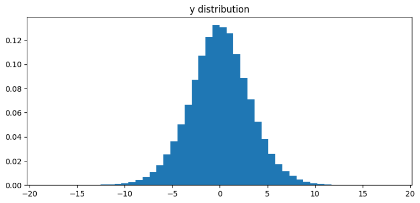
This is not what we want. What we want is unit Gaussian distributions throughout the layers of the neural net. The question is: how do we scale the w in such a way to preserve the unit Gaussian distribution in y?
Turns out you are supposed to divide w by the square root of the “fan-in” (number of input elements). In this case, since our w.
x = torch.randn(1000, 10)
w = torch.randn(10, 200) / 10**0.5
y = x @ w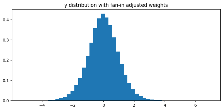
But what if we have a non-linear activation after the linear layer? How do we initialize the weights such that these activations take on reasonable values throughout the network?
Turns out there is a principled way to initialize these weights known as Kaiming initialization, introduced in the paper Delving Deep into Rectifiers. Basically our goal is to initialize weights such that std = gain / root(fan_mode), where fan_mode is either fan_in to preserve variance in the forward pass or fan_out for the backward pass. In the paper the analysis shows the difference between controlling either mode is about the same, so most people just use the default which is fan_in.
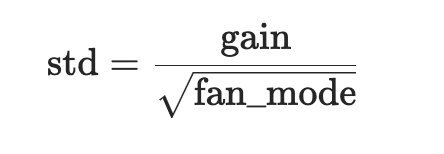
For every non-linearity, there is an associated “gain” multiplier, to counteract the “squashing” (lowering standard deviation) of non-linearities. The different gains can be found in the PyTorch docs.
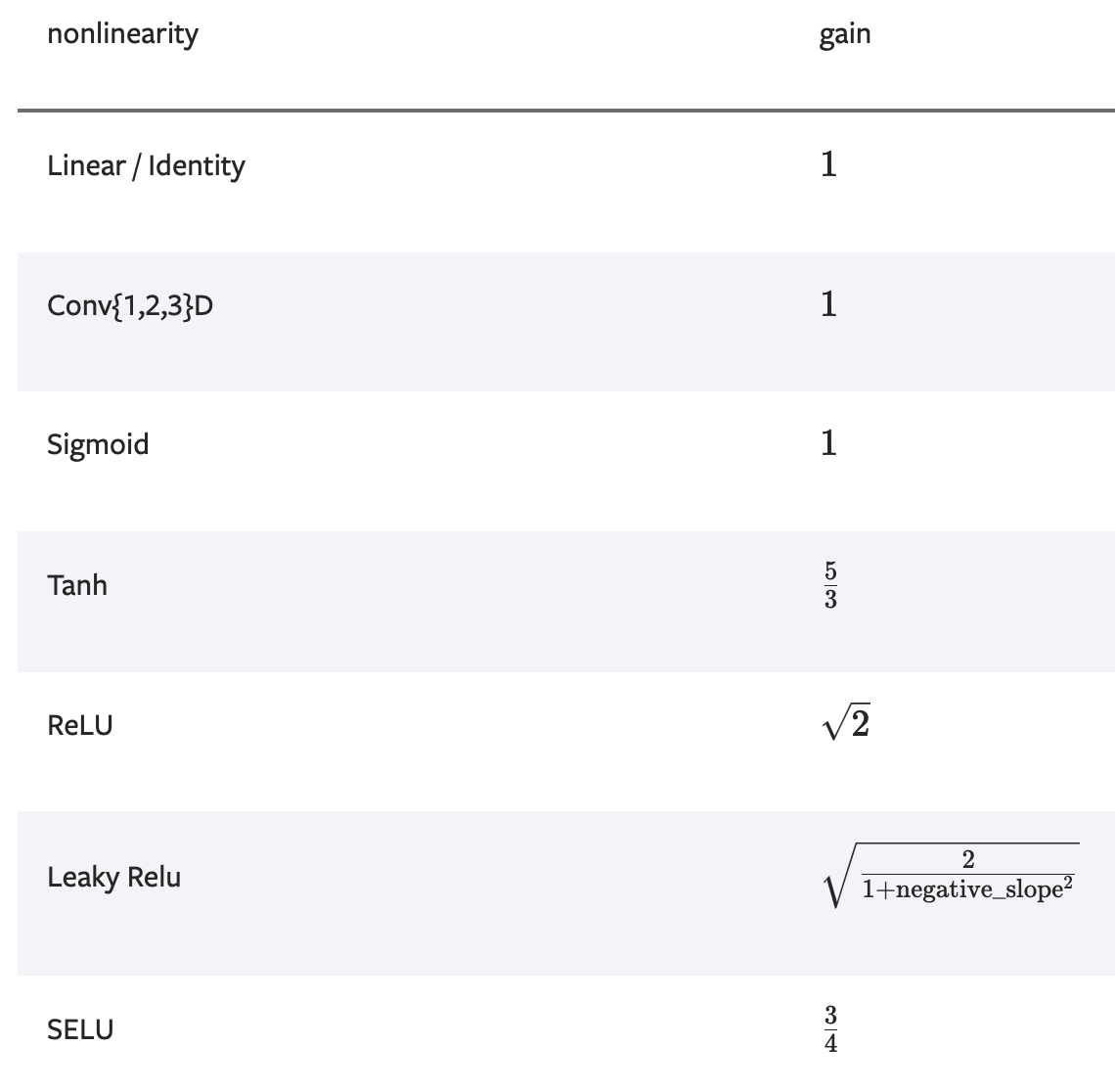
Back to our actual implementation. Because we are using tanh, we will use the gain of 5/3 and we will also be using the default fan_in mode. Setting the standard deviation of a unit gaussian is the same as just multiplying by the target number.
W1 = torch.randn((dimensions*block_size, neurons), generator=g) * 5/3 / (dimensions*block_size)**0.5Batch Normalization
So we have these hidden states, and we want them to be unit Gaussian, why not just make them exactly unit Gaussian (at least in the beginning)? That is the key idea of Batch Normalization introduced in the Batch Normalization paper.
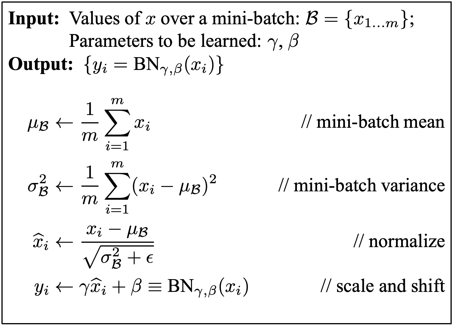
So instead of feeding hpreact directly into tanh, we just have to normalize it first. We will initialize bngain to 1 and bnbias to 0 so that we start with a unit Gaussian for hpreact. But as the network trains, it will be allowed to move the distribution around, allowing some neurons to be more active and others less active.
bngain = torch.ones((1, neurons))
bnbias = torch.zeros((1, neurons))
for i in range(training_steps):
# minibatch
batch_size = 32
ix = torch.randint(0, Xtr.shape[0], (batch_size,))
# forward pass
emb = C[Xtr[ix]]
embcat = emb.view(emb.shape[0], -1)
hpreact = embcat @ W1 + b1
bnmeani = hpreact.mean(0, keepdim=True)
bnstdi = hpreact.std(0, keepdim=True)
hpreact = bngain * (hpreact-bnmeani) / bnstdi + bnbias
h = torch.tanh(hpreact)In conclusion, Batch Normalization allows us to not have to worry about carefully tuning the initial weights of our neural net. Instead, we can just put a Batch Normalization layer after every linear layer.
The regularization effect of Batch Normalization
The stability of Batch Normalization comes at a cost. Instead of each example flowing through the neural net independently, we are coupling examples within the batches together. The activations of one example will now impact the activations of another because of the normalization across batches. Recall that we introduced mini batches just for efficiency and we never intended for this coupling.
However, in a somewhat round about way, this coupling of activations across randomly sampled batches actually has a beneficial regularization effect, discouraging the model from overfitting.
Batch normalization during inference
Another consequence of using Batch Normalization is that the forward pass now expects batches instead of examples. Instead of normalizing the activations based on the batch during inference, the paper suggest that we normalize based on the mean and standard deviation of the entire training set.
We can do this as a post-training step. But a more convenient way to do this is to keep a running mean and standard deviation during training loop. It’s important to note that these two values are not model parameters and so is outside of backpropagation and we don’t need PyTorch to compute the gradient for it.
bnmean_running = torch.zeros((1, neurons))
bnstd_running = torch.ones((1, neurons))
for i in range(training_steps):
    # minibatch
    batch_size = 32
    ix = torch.randint(0, Xtr.shape[0], (batch_size,))

    # forward pass
    emb = C[Xtr[ix]]
    embcat = emb.view(emb.shape[0], -1)
    hpreact = embcat @ W1 + b1
    bnmeani = hpreact.mean(0, keepdim=True)
    bnstdi = hpreact.std(0, keepdim=True)
    hpreact = bngain * (hpreact-bnmeani) / bnstdi + bnbias
        h = torch.tanh(hpreact)
# keep running mean and std for inference
with torch.no_grad():
bnmean_running = 0.999 * bnmean_running + 0.001 * bnmeani
bnstd_running = 0.999 * bnstd_running + 0.001 * bnstdiDuring inference, we will use the mean and std this way.
def split_loss(split):
    x, y = {
        'train': (Xtr, Ytr),
        'val': (Xdev, Ydev),
        'test': (Xte, Yte)
    }[split]
    emb = C[x]
    embcat = emb.view(emb.shape[0], -1)
    hpreact = embcat @ W1 + b1
    hpreact = bngain * (hpreact - bnmean_running) / bnstd_running + bnbias
    h = torch.tanh(hpreact)

    logits = h @ W2 + b2
    loss = F.cross_entropy(logits, y)
    print(f'{split} loss: {loss:.4f}')
A note on bias
If we have a batch normalization layer after a linear layer, the bias of the linear layer is actually not needed.
PyTorch Implementation
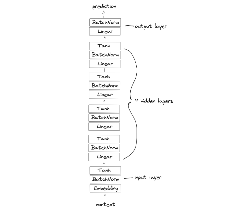
Let’s PyTorchify our model and make the network deeper! We will extract the initialization, forward, and backward logic of our layers so that we can easily scale our network without having to replicate our code.
class Linear:
    def __init__(self, fan_in, fan_out, bias=True):
        self.weight = torch.randn((fan_in, fan_out), generator=g) / fan_in**0.5
        self.bias = torch.zeros(fan_out) if bias else None

    def __call__(self, x):
        self.out = x @ self.weight
        if self.bias is not None:
            self.out += self.bias
        return self.out

    def parameters(self):
        return [self.weight] + ([self.bias] if self.bias is not None else [])

class BatchNorm1d:
    def __init__(self, dim, eps=1e-5, momentum=0.1):
        self.eps = eps
        self.momentum = momentum
        self.training = True
        # parameters (trained with backprop)
        self.gamma = torch.ones(dim)
        self.beta = torch.zeros(dim)
        # buffers (not trained with backprop)
        self.running_mean = torch.zeros(dim)
        self.running_var = torch.ones(dim)

    def __call__(self, x):
        # calculate the forward pass
        if self.training:
            # calculate the mean and variance on the batch
            xmean = x.mean(0, keepdim=True)
            xvar = x.var(0, keepdim=True)
        else:
            xmean = self.running_mean
            xvar = self.running_var
        # normalize the batch
        xhat = (x - xmean) / torch.sqrt(xvar + self.eps)
        self.out = self.gamma * xhat + self.beta
        # update the running mean and variance
        if self.training:
            with torch.no_grad():
                self.running_mean = (1-self.momentum) * self.running_mean + self.momentum * xmean
                self.running_var = (1-self.momentum) * self.running_var + self.momentum * xvar
        return self.out

    def parameters(self):
        return [self.gamma, self.beta]

class Tanh:
    def __call__(self, x):
        self.out = torch.tanh(x)
        return self.out
    def parameters(self):
        return []
n_emb = 10 # the dimension of the embedding
n_hidden = 100 # the number of neurons in the hidden layer of the MLP
g = torch.Generator().manual_seed(2147483647)
C = torch.randn((vocab_size, n_emb), generator=g)
layers = [
Linear(n_emb*block_size, n_hidden), BatchNorm1d(n_hidden), Tanh(),
Linear(n_hidden, n_hidden), BatchNorm1d(n_hidden), Tanh(),
Linear(n_hidden, n_hidden), BatchNorm1d(n_hidden), Tanh(),
Linear(n_hidden, n_hidden), BatchNorm1d(n_hidden), Tanh(),
Linear(n_hidden, n_hidden), BatchNorm1d(n_hidden), Tanh(),
Linear(n_hidden, vocab_size), BatchNorm1d(vocab_size),
]
with torch.no_grad():
# last layer: make less confident
layers[-1].weight *= 0.1
# layers[-1].weight *= 0.1
# all other layers: apply gain
for l in layers[:-1]:
if isinstance(l, Linear):
l.weight *= 5/3
parameters = [C] + [p for l in layers for p in l.parameters()]
print(sum(p.nelement() for p in parameters))
for p in parameters:
p.requires_grad_()
# same optimization as last time
max_steps = 200000
batch_size = 32
lossi = []
ud = []
for i in range(max_steps):
# minibatch construct
ix = torch.randint(0, Xtr.shape[0], (batch_size,), generator=g)
Xb, Yb = Xtr[ix], Ytr[ix] # batch X, Y
# forward pass
emb = C[Xb]
x = emb.view(emb.shape[0], -1)
for l in layers:
x = l(x)
loss = F.cross_entropy(x, Yb)
# backward pass
for layer in layers:
layer.out.retain_grad() # AFTER DEBUG: would take out retain_graph
for p in parameters:
p.grad = None
loss.backward()
# update
lr = 0.1 if i < (max_steps * 0.5) else 0.01
for p in parameters:
p.data -= lr * p.grad
# track stats
if i % 1000 == 0:
print(f'{i:6d}/{max_steps:6d}: {loss.item():.4f}')
lossi.append(loss.log10().item())
with torch.no_grad():
ud.append([(lr * p.grad.std() / p.data.std()).log10().item() for p in parameters])
break # AFTER DEBUG: would take out obviously to run full optimizationArchitecture
Visualizing layer activations
Let’s take a look at the activations for our new deeper model.
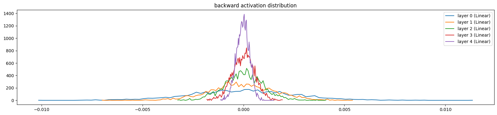
If we remove the BatchNorm and Tanh layers (leaving only Linear layers), we end up with a gain of 5/3 that is too high (since we don’t have the Tanh). This leads to the forward activations to get wider and wider, and the backward activations to get narrower and narrower.
layers = [
    Linear(n_emb*block_size, n_hidden),
    Linear(n_hidden, n_hidden),
    Linear(n_hidden, n_hidden),
    Linear(n_hidden, n_hidden),
    Linear(n_hidden, n_hidden),
    Linear(n_hidden, vocab_size),
]

with torch.no_grad():
    # last layer: make less confident
    layers[-1].weight *= 0.1
    # all other layers: apply gain
    for l in layers[:-1]:
        if isinstance(l, Linear):
            l.weight *= 5/3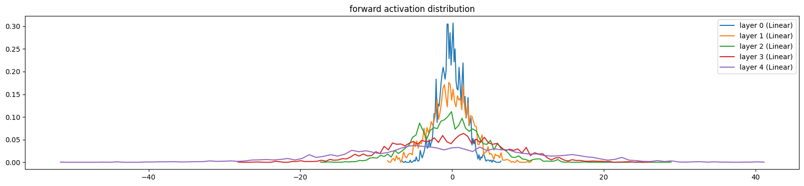
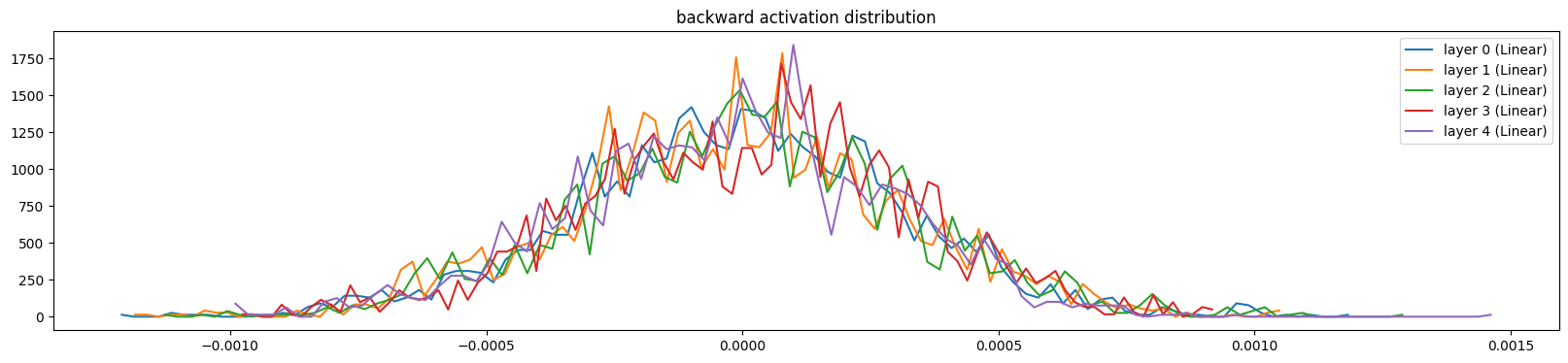
If we instead set the gain to 1.0 (the correct setting for no non-linearity), we end up with activations that look much better (stable across layers) for both forward and backwards.
layers = [
    Linear(n_emb*block_size, n_hidden),
    Linear(n_hidden, n_hidden),
    Linear(n_hidden, n_hidden),
    Linear(n_hidden, n_hidden),
    Linear(n_hidden, n_hidden),
    Linear(n_hidden, vocab_size),
]

with torch.no_grad():
    # last layer: make less confident
    layers[-1].weight *= 0.1
    # all other layers: apply gain
    for l in layers[:-1]:
        if isinstance(l, Linear):
            l.weight *= 1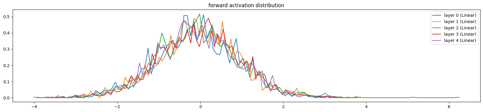
If we bring the Tanh layers back along with the gain of 5/3, then we will also see a nice plot of the activations. The shapes are different because we are now looking at the output of Tanh instead of Linear.
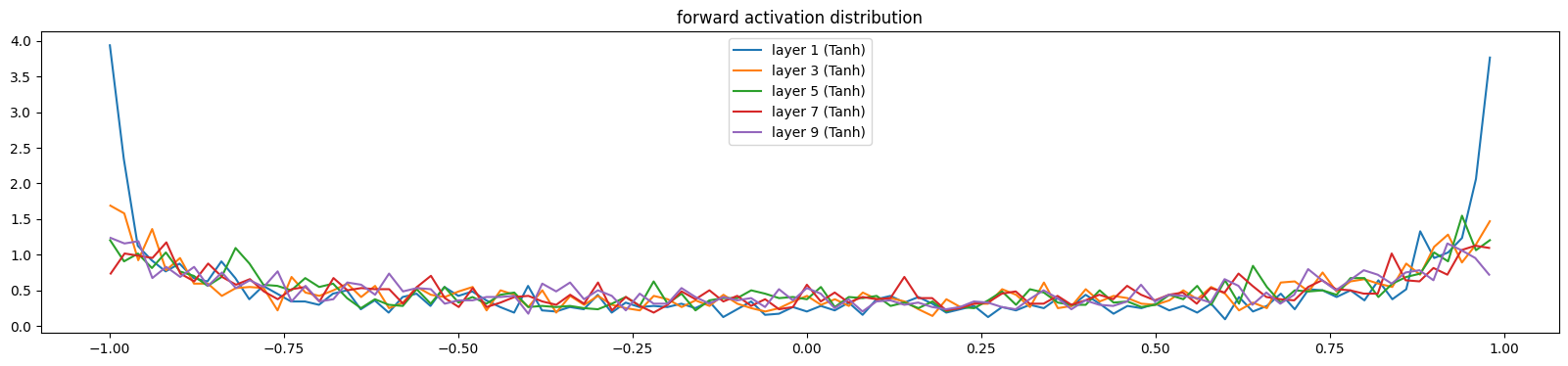
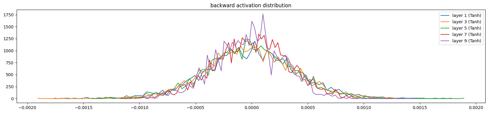
Gradient statistics
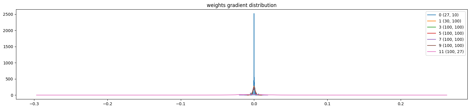
Another thing we can look at is the gradients of our parameters. This plot is a bit troubling since the final layer looks extremely wide, compared to all the other layers, at least at initialization. In other words, this final layer is being trained about 10x faster than all the other layers.
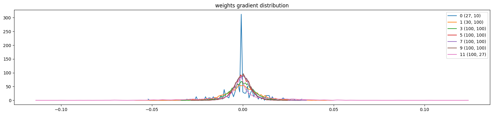
However, if we just let the training loop run for a few iterations (say 1000), the problem somewhat fixes itself. As you can see the last layer is coming in a bit.
Gradient update ratios
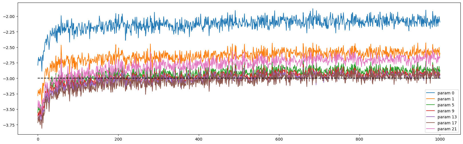
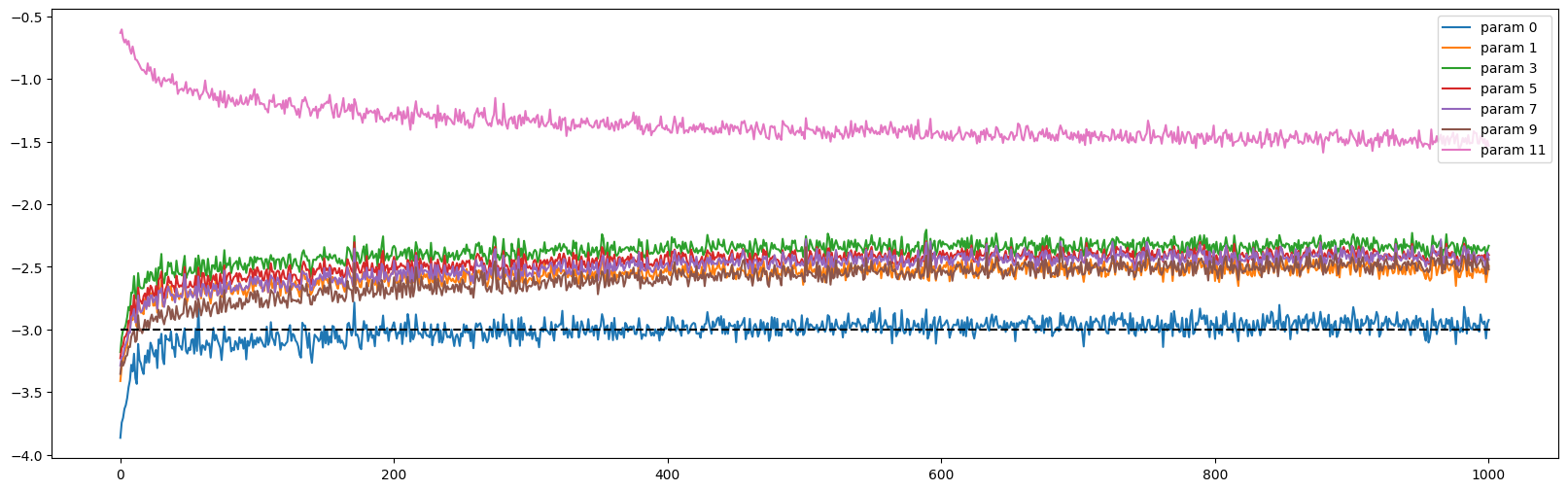
But perhaps what is more informative is looking at the update ratios (ie how fast our layers are training) over time.
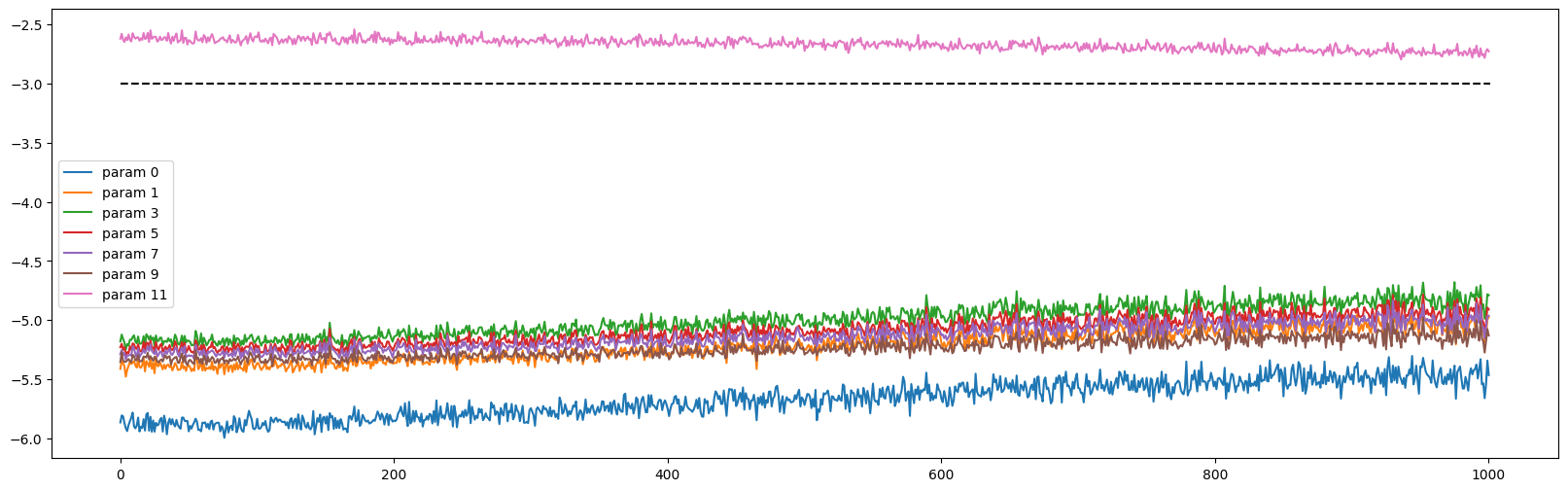
The black line is a benchmark set to ~1e-3 which is the recommended level.
If our learning rate is too low (say we set it to 0.001), then we can easily spot it using this chart.
Using these charts to spot problems
Let’s say we forgot to divide by the square root of fan-in in our linear layer weight initialization.
class Linear:
    def __init__(self, fan_in, fan_out, bias=True):
        self.weight = torch.randn((fan_in, fan_out), generator=g) # / fan_in**0.5
        self.bias = torch.zeros(fan_out) if bias else None
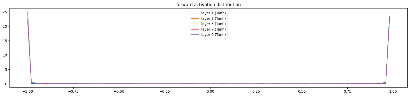
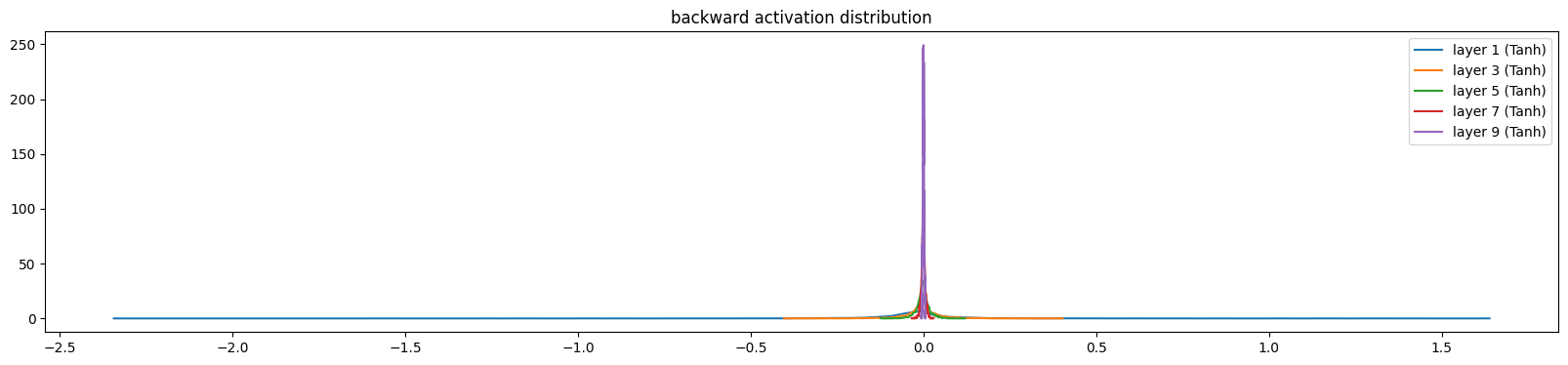
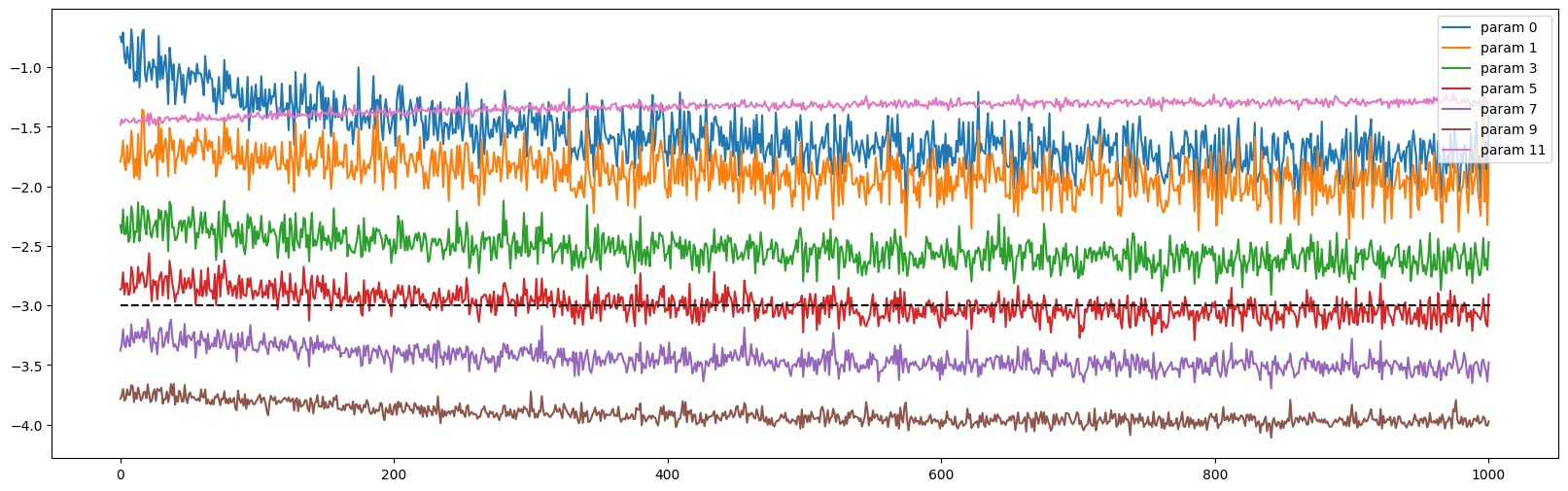
We will be able to quickly notice that something is wrong by looking at all of our charts. The forward activations are way too saturated. The backward activations go from extremely narrow to extremely wide. Same for the weights. We notice a lot of asymmetry across the layers in general.
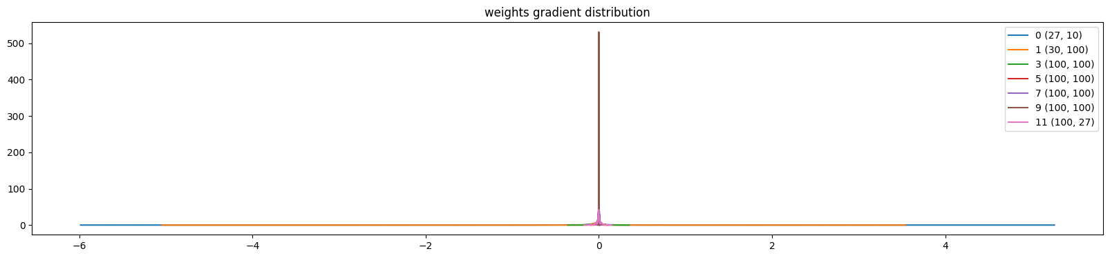
In this chart, we can see a lot of dispersion in terms of how fast each layer is learning, with some layers learning way too fast while others being too slow.
Batch Normalization
Above, we saw (again) how the network is somewhat sensitive to how we initialize the weights of the network without Batch Normalization. Adding Batch Normalization should make this more robust since it is forcing a normalization at the end of every linear layer.
For example, say we just didn’t do any of the weight initialization (don’t divide by sqrt of fan in for the linear layer, don’t set a gain). The network will still be completely fine.
class Linear:
    def __init__(self, fan_in, fan_out, bias=True):
        self.weight = torch.randn((fan_in, fan_out), generator=g) # / fan_in**0.5
        self.bias = torch.zeros(fan_out) if bias else None
layers = [
Linear(n_emb*block_size, n_hidden), BatchNorm1d(n_hidden), Tanh(),
Linear(n_hidden, n_hidden), BatchNorm1d(n_hidden), Tanh(),
Linear(n_hidden, n_hidden), BatchNorm1d(n_hidden), Tanh(),
Linear(n_hidden, n_hidden), BatchNorm1d(n_hidden), Tanh(),
Linear(n_hidden, n_hidden), BatchNorm1d(n_hidden), Tanh(),
Linear(n_hidden, vocab_size), BatchNorm1d(vocab_size),
]
with torch.no_grad():
# last layer: make less confident
layers[-1].gamma *= 0.1
# layers[-1].weight *= 0.1
# all other layers: apply gain
for l in layers[:-1]:
if isinstance(l, Linear):
l.weight *= 1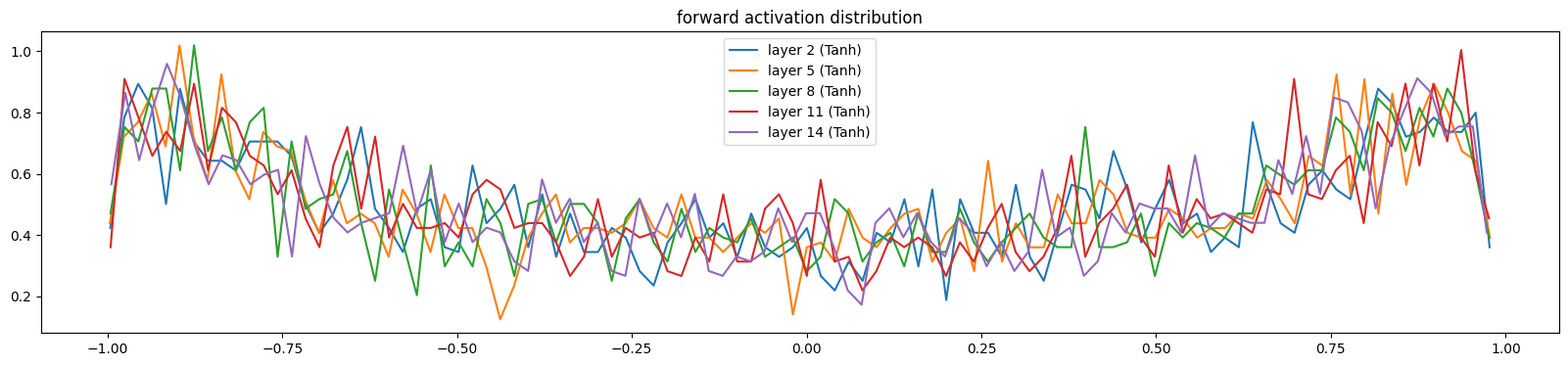
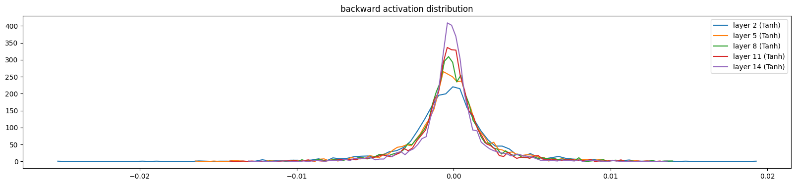
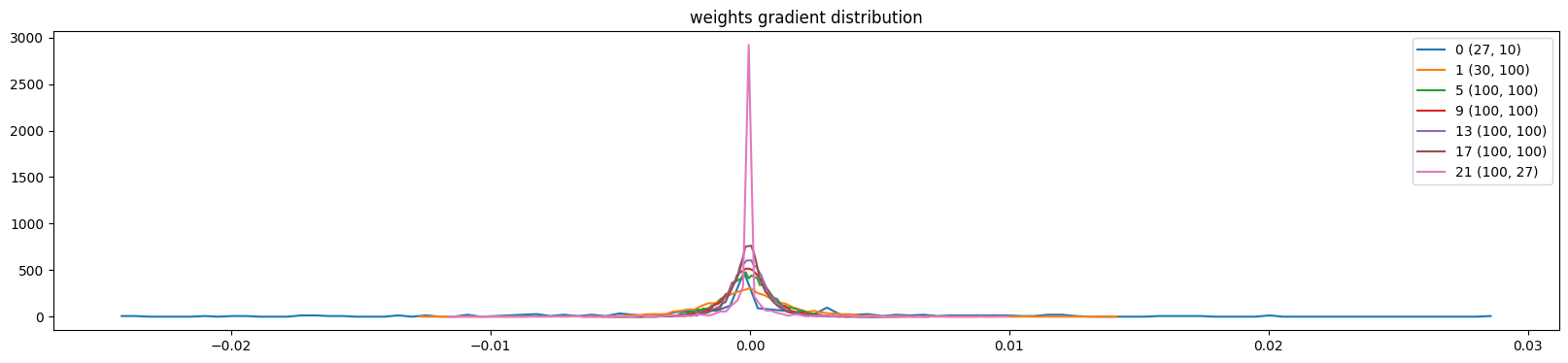
The only thing is that we may still need to re-tune our learning rates. So it is not a complete free pass. Here it looks like our learning rate is too low.
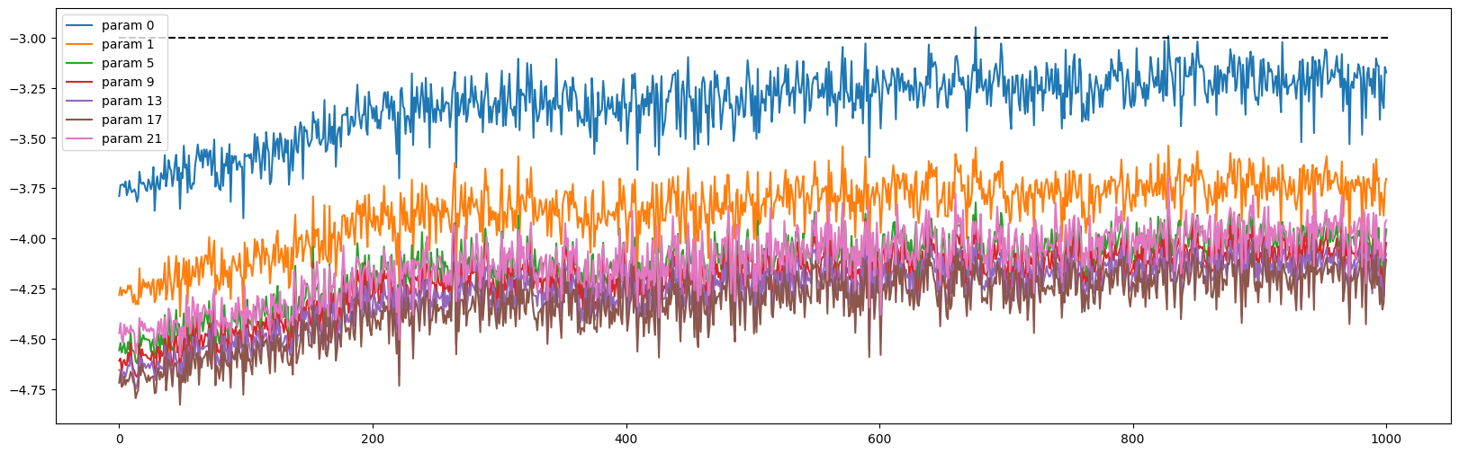
Bumping the learning rate from 0.1 to 1 looks good.