Makemore Part 4 - Becoming a Backprop Ninja

Introduction
As outlined in the medium post Yes you should understand backprop and in our previous lectures, it is important for us to understand how back propagation works at a deeper level than just calling PyTorch’s loss.backward.
So let’s replace the usage of loss.backward in our code and instead implement back propagation by hand!
Setup
To keep things simple, we will be revisiting our non-PyTorch implementation with just a single hidden layer. We will also just be focusing on a single pass on a single batch.
# input layer
emb = C[Xb]
embcat = emb.view(emb.shape[0], -1)

# hidden layer with batch normalization and tanh nonlinearity
hpreact = embcat @ W1 + b1
bnmeani = hpreact.mean(0, keepdim=True)
bnstdi = hpreact.std(0, keepdim=True)
hpreact = bngain * (hpreact-bnmeani) / bnstdi + bnbias
h = torch.tanh(hpreact)

# output layer
logits = h @ W2 + b2

# loss
loss = F.cross_entropy(logits, Yb)
First we need to rewrite our forward pass into smaller steps so that we can backward each step one at a time.
# input layer
emb = C[Xb] # embed the characters into vectors
embcat = emb.view(emb.shape[0], -1) # concatenate the vectors

# hidden layer with batch normalization and tanh nonlinearity
hprebn = embcat @ W1 + b1
bnmeani = 1/n*hprebn.sum(0, keepdim=True)
bndiff = hprebn - bnmeani
bndiff2 = bndiff**2
bnvar = 1/(n-1)*(bndiff2).sum(0, keepdim=True)
bnvar_inv = (bnvar + 1e-5)**-0.5
bnraw = bndiff * bnvar_inv
hpreact = bngain * bnraw + bnbias
h = torch.tanh(hpreact)

# output layer
logits = h @ W2 + b2

# loss
logit_maxes = logits.max(1, keepdim=True).values
norm_logits = logits - logit_maxes
counts = norm_logits.exp()
counts_sum = counts.sum(1, keepdims=True)
counts_sum_inv = counts_sum**-1
probs = counts * counts_sum_inv
logprobs = probs.log()
loss = -logprobs[range(n), Yb].mean()
Exercise 1: Backprop by hand
# utility function we will use later when comparing manual gradients to PyTorch gradients
def cmp(s, dt, t):
  ex = torch.all(dt == t.grad).item()
  app = torch.allclose(dt, t.grad)
  maxdiff = (dt - t.grad).abs().max().item()
  print(f'{s:15s} | exact: {str(ex):5s} | approximate: {str(app):5s} | maxdiff: {maxdiff}')
# Exercise 1: backprop through the whole thing manually,
# backpropagating through exactly all of the variables
# as they are defined in the forward pass above, one by one
# loss = -logprobs[range(n), Yb].mean()
# what is the derivative of mean? --> mean is just addition and division, derivative of divide is just 1/x, where x is the count
# why do i need to multiply by the one hot to change shape though? --> because of logprobs[range(n), Yb] is picking out row 1-2 at column Yb
dlogprobs = -F.one_hot(Yb, num_classes=27).float() * torch.tensor(1.0 / len(logprobs))
cmp('logprobs', dlogprobs, logprobs)
# logprobs = probs.log()
# derivative of log x is 1/x
dprobs = 1/probs * dlogprobs
cmp('probs', dprobs, probs)
# probs = counts * counts_sum_inv
# derivative of multiply is just the other thing
# why do i need to sum to change the shape though? probably because of the broadcasting rules?
dcounts_sum_inv = (dprobs * counts).sum(1, keepdims=True)
cmp('counts_sum_inv', dcounts_sum_inv, counts_sum_inv)
# counts_sum_inv = counts_sum**-1
# derivative of x^-1 is -1/x^2
dcounts_sum = (-counts_sum**-2) * dcounts_sum_inv
cmp('counts_sum', dcounts_sum, counts_sum)
# counts_sum = counts.sum(1, keepdims=True)
# derivative of sum is just 1
# probs = counts * counts_sum_inv
# derivative of multiply is just the other thing
# since counts is used twice, we need to add the gradients together
dcounts = torch.ones_like(counts) * dcounts_sum
dcounts += dprobs * counts_sum_inv
cmp('counts', dcounts, counts)
# counts = norm_logits.exp()
# derivative of exp is exp
dnorm_logits = norm_logits.exp() * dcounts
cmp('norm_logits', dnorm_logits, norm_logits)
# norm_logits = logits - logit_maxes
# derivative of subtract is just -1
dlogit_maxes = -dnorm_logits.sum(1, keepdims=True)
cmp('logit_maxes', dlogit_maxes, logit_maxes)
# logit_maxes = logits.max(1, keepdim=True).values
# norm_logits = logits - logit_maxes
dlogits = F.one_hot(logits.max(1).indices, num_classes=27).float() * dlogit_maxes
dlogits += dnorm_logits
cmp('logits', dlogits, logits)
# logits = h @ W2 + b2
dh = dlogits @ W2.T
cmp('h', dh, h)
dW2 = h.T @ dlogits
cmp('W2', dW2, W2)
db2 = dlogits.sum(0)
cmp('b2', db2, b2)
# h = torch.tanh(hpreact)
# derivative of tanh is 1 - tanh^2
dhpreact = (1 - h**2) * dh
cmp('hpreact', dhpreact, hpreact)
# hpreact = bngain * bnraw + bnbias
# this is element wise multiplication, not matrix multiplication!
dbngain = (bnraw * dhpreact).sum(0, keepdims=True)
dbnraw = bngain * dhpreact
dbnbias = dhpreact.sum(0, keepdims=True)
cmp('bngain', dbngain, bngain)
cmp('bnbias', dbnbias, bnbias)
cmp('bnraw', dbnraw, bnraw)
dbnvar_inv = (bndiff * dbnraw).sum(0, keepdims=True)
cmp('bnvar_inv', dbnvar_inv, bnvar_inv)
# bnvar_inv = (bnvar + 1e-5)**-0.5
# derivative of x^-0.5 is -0.5*x^-1.5
dbnvar = (-0.5*(bnvar + 1e-5)**-1.5) * dbnvar_inv
cmp('bnvar', dbnvar, bnvar)
# bnvar = 1/(n-1)*(bndiff2).sum(0, keepdim=True)
dbndiff2 = torch.ones_like(bndiff2) * (1/(n-1)) * dbnvar
cmp('bndiff2', dbndiff2, bndiff2)
# bnraw = bndiff * bnvar_inv
# again, element wise multiplication
dbndiff = bnvar_inv * dbnraw
dbndiff += 2 * bndiff * dbndiff2
cmp('bndiff', dbndiff, bndiff)
# bndiff = hprebn - bnmeani
# bnmeani = 1/n*hprebn.sum(0, keepdim=True)
dbnmeani = -dbndiff.sum(0, keepdims=True)
dhprebn = dbndiff.clone()
dhprebn += 1/n * dbnmeani
cmp('bnmeani', dbnmeani, bnmeani)
cmp('hprebn', dhprebn, hprebn)
# hprebn = embcat @ W1 + b1
dembcat = dhprebn @ W1.T
cmp('embcat', dembcat, embcat)
dW1 = embcat.T @ dhprebn
cmp('W1', dW1, W1)
db1 = dhprebn.sum(0)
cmp('b1', db1, b1)
# embcat = emb.view(emb.shape[0], -1)
demb = dembcat.view(emb.shape)
cmp('emb', demb, emb)
# emb = C[Xb]
dC = torch.zeros_like(C)
for k in range(Xb.shape[0]):
for j in range(Xb.shape[1]):
dC[Xb[k,j]] += demb[k,j]
cmp('C', dC, C)Everything above is pretty straightforward in terms of how the derivatives are derived. The only things worth mentioning is that we need to be very careful about broadcasting, and that we need to make sure we accumulate gradients when a term is used multiple times.
Derivative of matrix multiplication
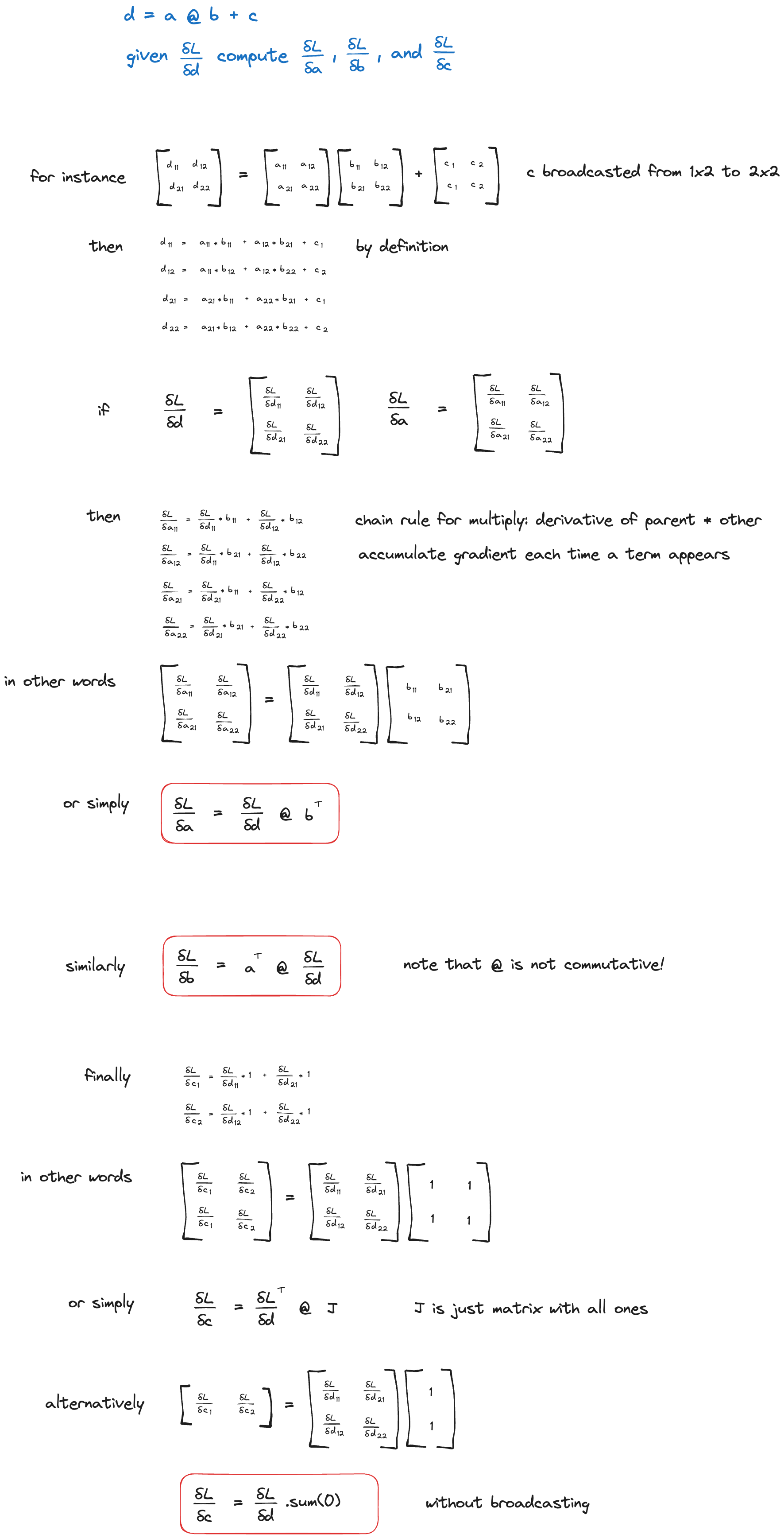
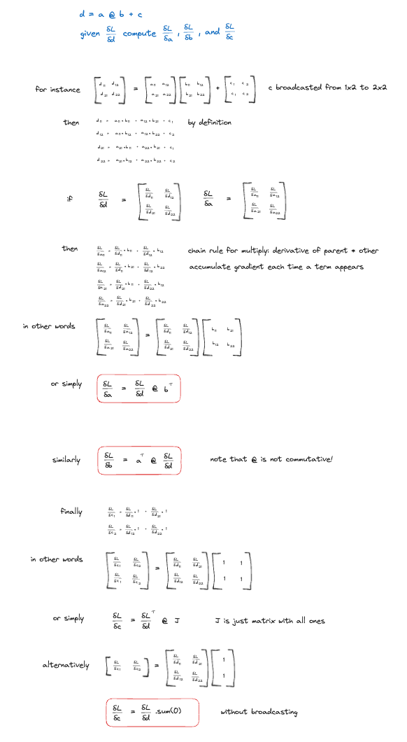
The only thing that is a bit complicated is how we actually find the derivative of the matrix multiplication in the linear layer. We will go through a toy example to help us understand the general principle.
I will just put my final work here. My full notes can be found here.
Exercise 2: Back propagating cross entropy analytically
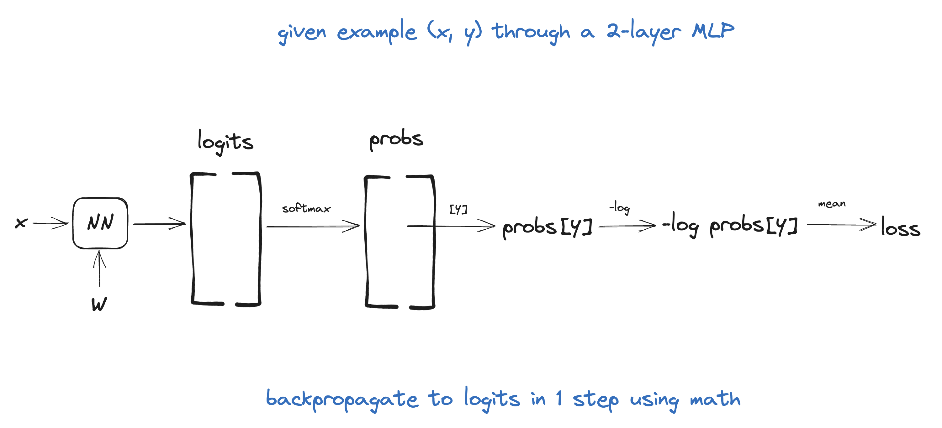
So instead of implementing the cross entropy loss manually, we would normally just call the PyTorch implementation.
# cross entropy loss manual
logit_maxes = logits.max(1, keepdim=True).values
norm_logits = logits - logit_maxes
counts = norm_logits.exp()
counts_sum = counts.sum(1, keepdims=True)
counts_sum_inv = counts_sum**-1
probs = counts * counts_sum_inv
logprobs = probs.log()
loss = -logprobs[range(n), Yb].mean()
# cross entropy loss one-liner with PyTorch
loss_fast = F.cross_entropy(logits, Yb)Math
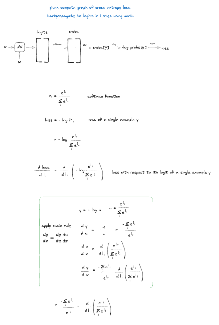
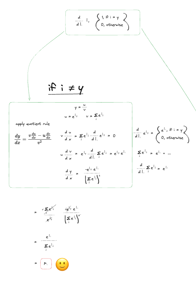
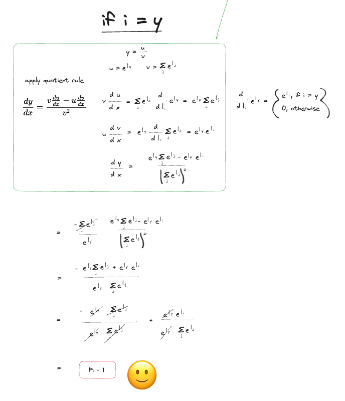
Again I will only put my final work here, full notes can be found in this post.
Code
All of that math allows us to simplify the backward pass of the cross entropy loss to just this!
dlogits = F.softmax(logits, 1)
dlogits[range(n), Yb] -= 1
dlogits /= n
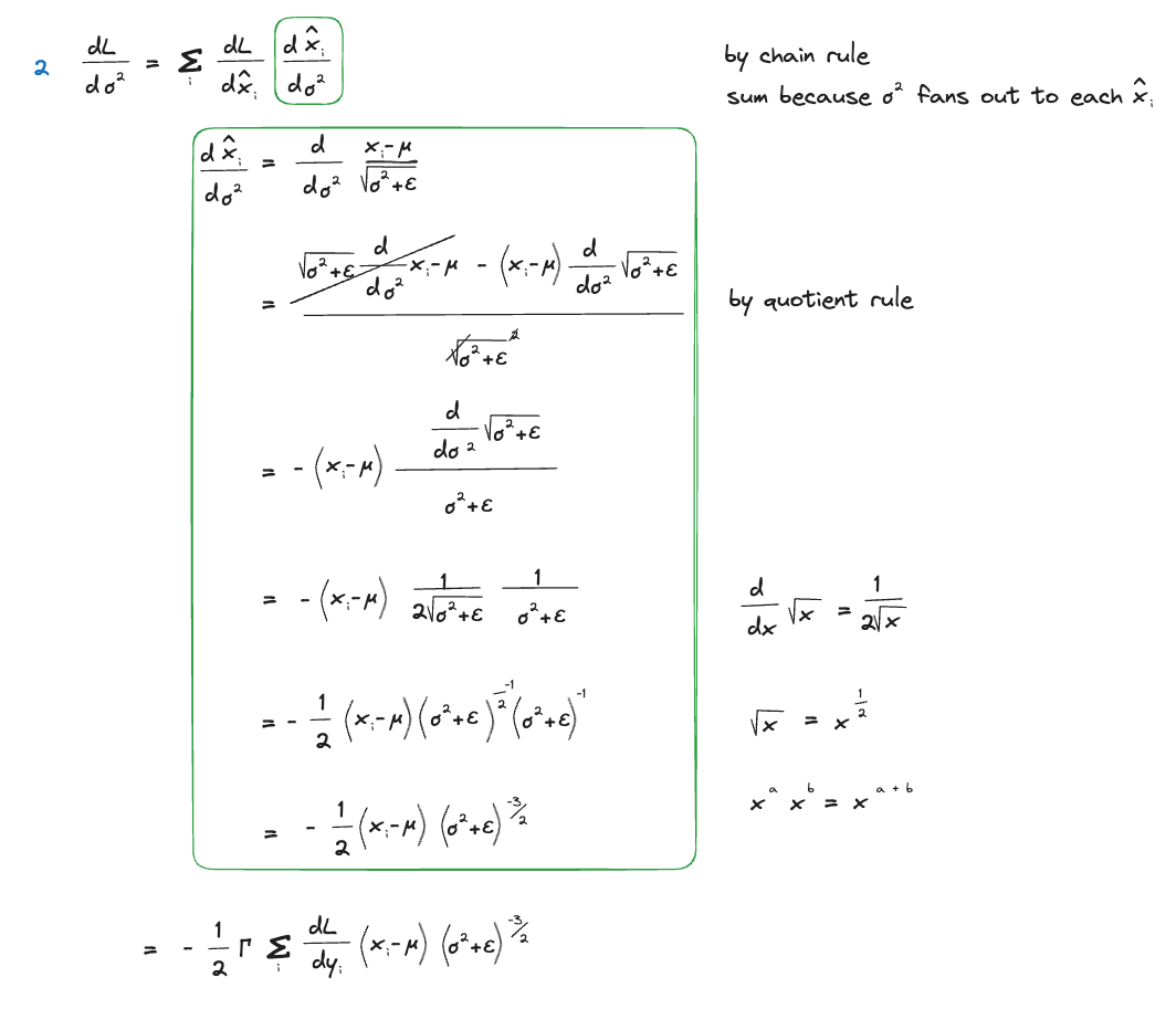
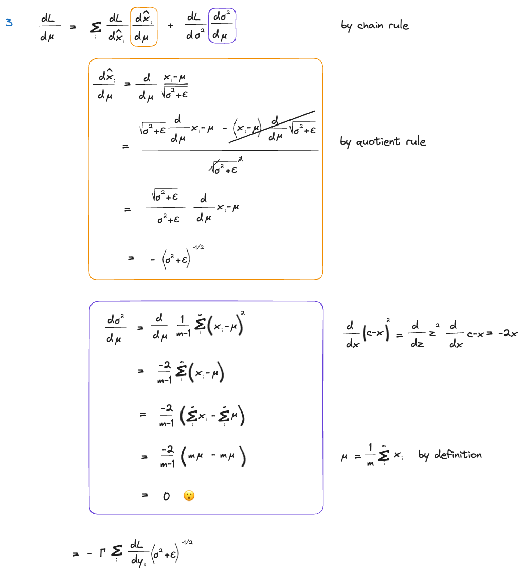
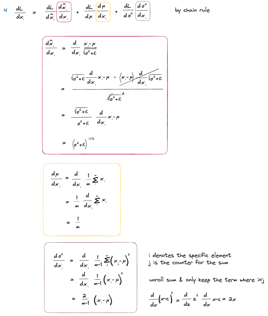
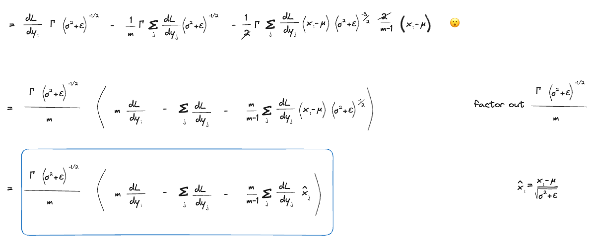
Exercise 3: Back propagating batch normalization analytically
So instead of implementing the batch normalization in many steps, we can implement it in this one line. Again, our goal is to then derive the derivative of this one-liner analytically.
# Batch normalization manual
bnmeani = 1/n*hprebn.sum(0, keepdim=True)
bndiff = hprebn - bnmeani
bndiff2 = bndiff**2
bnvar = 1/(n-1)*(bndiff2).sum(0, keepdim=True)
bnvar_inv = (bnvar + 1e-5)**-0.5
bnraw = bndiff * bnvar_inv
hpreact = bngain * bnraw + bnbias
# Batch normalization one-liner
hpreact_fast = bngain * (hprebn - hprebn.mean(0, keepdim=True)) / torch.sqrt(hprebn.var(0, keepdim=True, unbiased=True) + 1e-5) + bnbiasMath
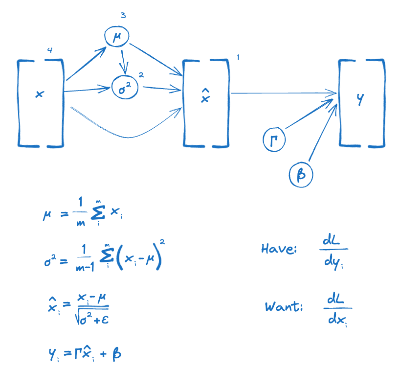
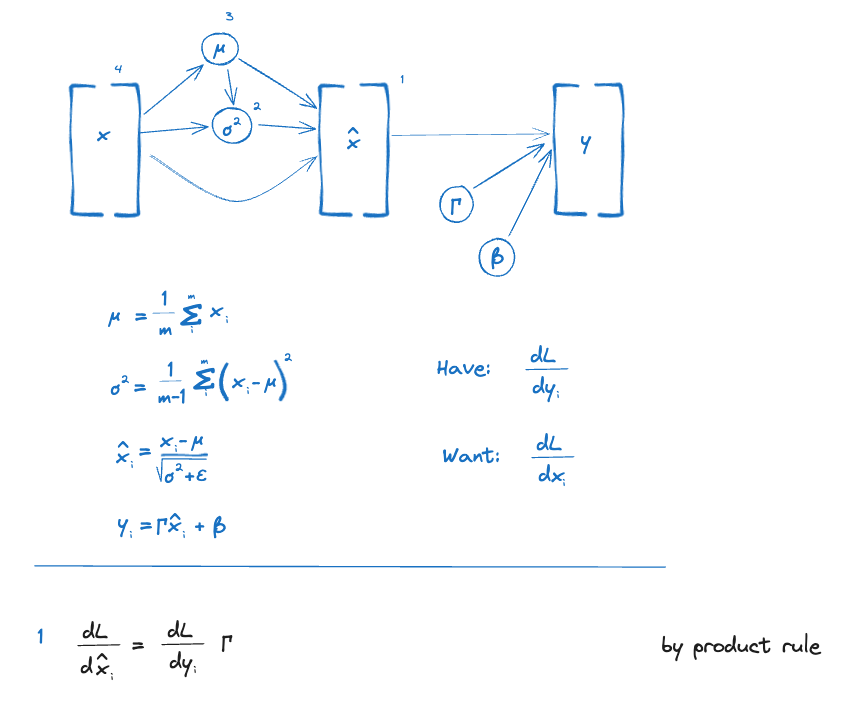
I will only show my final result here, full notes can be found in this post.
Code
All of the math above allows us to simplify the backwards pass of batch normalization to this one line!
dhprebn = bngain*bnvar_inv/n * (n*dhpreact - dhpreact.sum(0) - n/(n-1)*bnraw*(dhpreact*bnraw).sum(0))Exercise 4: Putting it all together
Alright, after all of that fun, we are now able to finally remove the usage of loss.backward in our code!
# Exercise 4: putting it all together!
# Train the MLP neural net with your own backward pass

# init
n_embd = 10 # the dimensionality of the character embedding vectors
n_hidden = 200 # the number of neurons in the hidden layer of the MLP

g = torch.Generator().manual_seed(2147483647) # for reproducibility
C  = torch.randn((vocab_size, n_embd),            generator=g)
# Layer 1
W1 = torch.randn((n_embd * block_size, n_hidden), generator=g) * (5/3)/((n_embd * block_size)**0.5)
b1 = torch.randn(n_hidden,                        generator=g) * 0.1
# Layer 2
W2 = torch.randn((n_hidden, vocab_size),          generator=g) * 0.1
b2 = torch.randn(vocab_size,                      generator=g) * 0.1
# BatchNorm parameters
bngain = torch.randn((1, n_hidden))*0.1 + 1.0
bnbias = torch.randn((1, n_hidden))*0.1

parameters = [C, W1, b1, W2, b2, bngain, bnbias]
print(sum(p.nelement() for p in parameters)) # number of parameters in total
for p in parameters:
  p.requires_grad = True

# same optimization as last time
max_steps = 200000
batch_size = 32
n = batch_size # convenience
lossi = []

# use this context manager for efficiency once your backward pass is written (TODO)
with torch.no_grad():

  # kick off optimization
  for i in range(max_steps):

    # minibatch construct
    ix = torch.randint(0, Xtr.shape[0], (batch_size,), generator=g)
    Xb, Yb = Xtr[ix], Ytr[ix] # batch X,Y

    # forward pass
    emb = C[Xb] # embed the characters into vectors
    embcat = emb.view(emb.shape[0], -1) # concatenate the vectors
    # Linear layer
    hprebn = embcat @ W1 + b1 # hidden layer pre-activation
    # BatchNorm layer
    # -------------------------------------------------------------
    bnmean = hprebn.mean(0, keepdim=True)
    bnvar = hprebn.var(0, keepdim=True, unbiased=True)
    bnvar_inv = (bnvar + 1e-5)**-0.5
    bnraw = (hprebn - bnmean) * bnvar_inv
    hpreact = bngain * bnraw + bnbias
    # -------------------------------------------------------------
    # Non-linearity
    h = torch.tanh(hpreact) # hidden layer
    logits = h @ W2 + b2 # output layer
    loss = F.cross_entropy(logits, Yb) # loss function

    # backward pass
    for p in parameters:
      p.grad = None
    # loss.backward() # use this for correctness comparisons, delete it later!

    # manual backprop! #swole_doge_meme
    # -----------------
    dlogits = F.softmax(logits, 1)
    dlogits[range(n), Yb] -= 1
    dlogits /= n
    # 2nd layer backprop
    dh = dlogits @ W2.T
    dW2 = h.T @ dlogits
    db2 = dlogits.sum(0)
    # tanh
    dhpreact = (1 - h**2) * dh
    # batch norm backprop
    dbngain = (bnraw * dhpreact).sum(0, keepdims=True)
    dbnraw = bngain * dhpreact
    dbnbias = dhpreact.sum(0, keepdims=True)
    dhprebn = bngain*bnvar_inv/n * (n*dhpreact - dhpreact.sum(0) - n/(n-1)*bnraw*(dhpreact*bnraw).sum(0))
    # 1st layer
    dembcat = dhprebn @ W1.T
    dW1 = embcat.T @ dhprebn
    db1 = dhprebn.sum(0)
    # embedding
    demb = dembcat.view(emb.shape)
    dC = torch.zeros_like(C)
    for k in range(Xb.shape[0]):
        for j in range(Xb.shape[1]):
            dC[Xb[k,j]] += demb[k,j]

    grads = [dC, dW1, db1, dW2, db2, dbngain, dbnbias]
    # -----------------

    # update
    lr = 0.1 if i < 100000 else 0.01 # step learning rate decay
    for p, grad in zip(parameters, grads):
      # p.data += -lr * p.grad # old way of cheems doge (using PyTorch grad from .backward())
      p.data += -lr * grad # new way of swole doge TODO: enable

    # track stats
    if i % 10000 == 0: # print every once in a while
      print(f'{i:7d}/{max_steps:7d}: {loss.item():.4f}')
    lossi.append(loss.log10().item())

    # if i >= 100: # TODO: delete early breaking when you're ready to train the full net
    #   break