Makemore Part 5 - Building a WaveNet

2023-11 · notes · zero to hero

Building makemore Part 5: Building a WaveNet

Overview

We take the 2-layer MLP from part 3 and we make it deeper with a tree-like structure (instead of just stacking more layers like we did before).

Some code improvements

Starter Code

Here is the Torchified 2-layer MLP from before. I won’t include the class definitions of our Linear, BatchNorm1d, Tanh building blocks here since they haven’t changed.

block_size = 3 # context length: how many characters do we take to predict the next one?
n_embd = 10 # the dimensionality of the character embedding vectors
n_hidden = 200 # the number of neurons in the hidden layer of the MLP
C = torch.randn((vocab_size, n_embd))
layers = [
  Linear(n_embd * block_size, n_hidden, bias=False), BatchNorm1d(n_hidden), Tanh(),
  Linear(n_hidden, vocab_size),
]

# parameter init
with torch.no_grad():
  layers[-1].weight *= 0.1 # last layer make less confident

parameters = [C] + [p for layer in layers for p in layer.parameters()]
print(sum(p.nelement() for p in parameters)) # number of parameters in total
for p in parameters:
  p.requires_grad = True

# same optimization as last time
max_steps = 200000
batch_size = 32
lossi = []

for i in range(max_steps):

  # minibatch construct
  ix = torch.randint(0, Xtr.shape[0], (batch_size,))
  Xb, Yb = Xtr[ix], Ytr[ix] # batch X,Y

  # forward pass
  emb = C[Xb]
  x = emb.view(emb.shape[0], -1)
  for layer in layers:
    x = layer(x)
  loss = F.cross_entropy(x, Yb)

  # backward pass
  for p in parameters:
    p.grad = None
  loss.backward()

  # update: simple SGD
  lr = 0.1 if i < 150000 else 0.01 # step learning rate decay
  for p in parameters:
    p.data += -lr * p.grad

  # track stats
  if i % 10000 == 0: # print every once in a while
    print(f'{i:7d}/{max_steps:7d}: {loss.item():.4f}')
  lossi.append(loss.log10().item())

Fixing the learning rate plot

This is what our original plot of our looks like. But it is kind of difficult to read given how wide the band of values are. The wide distribution of values come from the fact that we are training in batches.

plt.plot(lossi)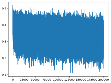

Instead of plotting each datapoint, we can plot the mean of each 1000 points to get a smoother line. This plot is much more informative. We can even start to see the effect of our learning rate decay, which was previously completely obfuscated by the wide band of values.

plt.plot(torch.tensor(lossi).view(-1, 1000).mean(1))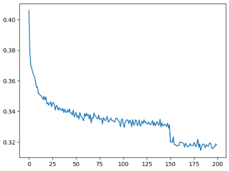

Pytorchifying the embedding

In order to clean up our code a bit, we can introduce these two classes to replace the special case code we have for our embedding.

class Embedding:
  def __init__(self, num_embeddings, embedding_dim):
    self.weight = torch.randn((num_embeddings, embedding_dim))

  def __call__(self, IX):
    self.out = self.weight[IX]
    return self.out

  def parameters(self):
    return [self.weight]

class Flatten:
  def __call__(self, x):
    self.out = x.view(x.shape[0], -1)
    return self.out

  def parameters(self):
    return []

Instead of having to declare C outside of layers, and then having to add C into our parameters and then having to manually do the flattening inside the forward pass, the embedding and flattening operation can just become a layer

layers = [
  Embedding(vocab_size, n_embd), Flatten(),
  Linear(n_embd * block_size, n_hidden, bias=False), BatchNorm1d(n_hidden), Tanh(),
  Linear(n_hidden, vocab_size),
]

parameters = [p for layer in layers for p in layer.parameters()]

And the forward pass becomes nice and uniform

# foward pass
for layer in layers:
    x = layer(x)

Pytorchifying the model

Instead of having to maintain a list of layers, and having to for-loop over them in various places, we can wrap our layers inside of a “container” called Sequential.

class Sequential:
  def __init__(self, layers):
    self.layers = layers

  def __call__(self, x):
    for layer in self.layers:
      x = layer(x)
    self.out = x
    return self.out

  def parameters(self):
    # get parameters of all layers and stretch them out into one list
    return [p for layer in self.layers for p in layer.parameters()]

Instead of a raw layers array, we now have a models object

model = Sequential([
   Embedding(vocab_size, n_embd), Flatten(),
   Linear(n_embd * 8, n_hidden, bias=False), BatchNorm1d(n_hidden), Tanh(),
   Linear(n_hidden, vocab_size),
])

with torch.no_grad():
   model.layers[-1].weight *= 0.1 # last layer make less confident

Which simplifies our forward pass to just 2 lines

# forward pass
logits = model(Xb)
loss = F.cross_entropy(logits, Yb) # loss function

Wavenet

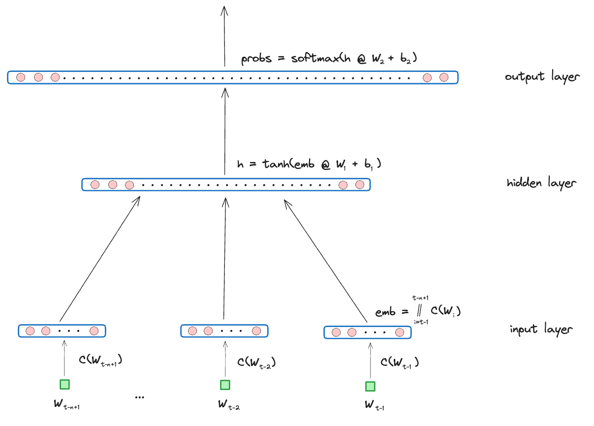
Recall the architecture of our initial MLP.

And then recall how we tried to make it deeper by adding more hidden layers.

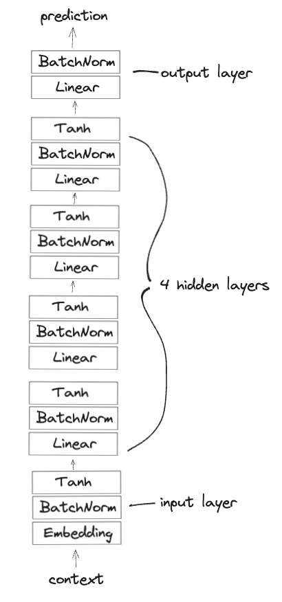
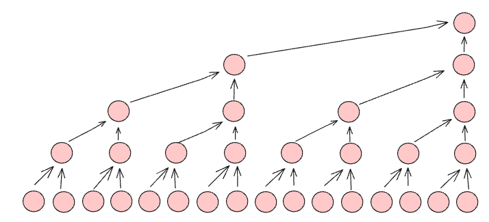
But even though we are adding more hidden layers, we are still “crushing” the context of the input layer too soon, which limits our ability to increase the context length.

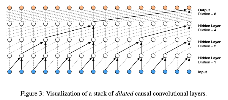
Instead, we want to fuse the earlier layers together progressively (or hierarchically) like they did in the Wavenet paper.

WaveNet: A Generative Model for Raw Audio

Batch dimensions

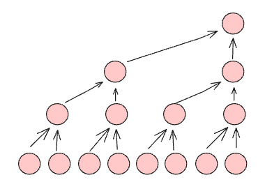
For us, we will be increasing our block_size from 3 to 8, which makes our graph look like this.

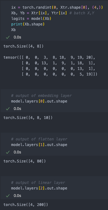
Say we have a batch of 4 examples, let’s try to visualize the shapes of the tensors through the forward pass.

block_size = 8
n_embd = 10
n_hidden = 200

model = Sequential([
   Embedding(vocab_size, n_embd), Flatten(),
   Linear(n_embd * 8, n_hidden, bias=False), BatchNorm1d(n_hidden), Tanh(),
   Linear(n_hidden, vocab_size),
])

Let’s say we have a hypothetical batch of 4 examples.

• Xb is 4 examples x 8 characters
• output of embedding is 4 examples x 8 characters x 10 embedding dimensions where each character got turned into a 10 dimension vector
• output of flatten is 4 examples x 80 character embeddings where the embeddings of all 8 characters got flattened or concatenated into a single array
• output of linear layer is 4 examples x 200 neurons otherwise known as 200 “channels”

What happens inside the linear layer looks like this. 4 is our batch dimension and 80 is the dimension of the input. Since we have 200 channels, we end up with 4x200 as our output.

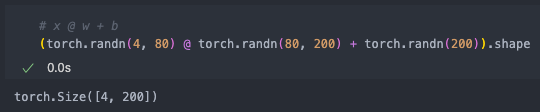
But we can actually add more batch dimensions. For example if we added 2 more batch dimensions so that our input was 4x5x6 then our output will just be 4x5x6x200. Essentially the matrix multiplication only happens on the last dimension of the input, and all preceding dimensions are treated as batch dimensions and simply passes through.

This is useful because we can essentially break up the 8 characters of each example into, say, 4 groups of 2 characters, and our linear layer would still work as expected. This is

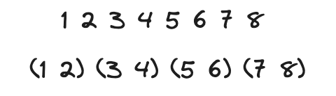
So instead of having 4x80 as our input, we can actually rewrite this as 4x4x20 where the first 4 is our initial batch dimension, and the 80 (which was 8 characters x 10 dimensions) got split into 4x20 (which is 4 groups of 2 characters x 10 dimensions).

Flatten Consecutive

Recall that we have this Flatten layer. Basically all it does is keep the first (or zeroth) dimension and flatten the rest of the dimensions. So a 4x8x10 would become 4x80.

class Flatten:
  def __call__(self, x):
    self.out = x.view(x.shape[0], -1)
    return self.out

  def parameters(self):
    return []

What we want is a Flatten that can turn 4x8x10 into 4x4x20 More specifically, we want this Flatten to keep the 4 batch dimension, but group the 8x10 dimensions into groups of 2, which would become 4x20. If the 2nd dimension becomes 1, then we “squeeze” it to remove the dimension completely. We call this FlattenConsecutive.

class FlattenConsecutive:
  def __init__(self, n):
    self.n = n

  def __call__(self, x):
    B, T, C = x.shape
    x = x.view(B, T//self.n, C*self.n)
    if x.shape[1] == 1:
      x = x.squeeze(1)
    self.out = x
    return self.out

  def parameters(self):
    return []

Calling FlattenConsecutive(8) would yield the same result as our original flatten. Since we are grouping a 4x8x10 into groups of 8, we get 4x1x80, and we squeeze the 2nd dimension away to get 4x80.

block_size = 8
n_embd = 10
n_hidden = 200
model = Sequential([
  Embedding(vocab_size, n_embd),
  FlattenConsecutive(block_size), Linear(n_embd * block_size, n_hidden, bias=False), BatchNorm1d(n_hidden), Tanh(),
  Linear(n_hidden, vocab_size),
])

If we want to progressively fuse by 2 over 4 hidden layers, we can just copy and paste the linear layer sandwich. Note that the hidden layers now have a fan-in of n_hidden*2 instead of just n_hidden since we stuck a FlattenConsecutive in front of it.

block_size = 8
n_embd = 10
n_hidden = 200
group_size = 2
model = Sequential([
  Embedding(vocab_size, n_embd),
  FlattenConsecutive(group_size), Linear(n_embd * group_size, n_hidden, bias=False), BatchNorm1d(n_hidden), Tanh(),
  FlattenConsecutive(group_size), Linear(n_hidden*group_size, n_hidden, bias=False), BatchNorm1d(n_hidden), Tanh(),
  FlattenConsecutive(group_size), Linear(n_hidden*group_size, n_hidden, bias=False), BatchNorm1d(n_hidden), Tanh(),
  Linear(n_hidden, vocab_size),
])

If we inspect the shapes of the output of each layer…

• Embedding: 4x8x10 (batch of 4, 8 characters each, 10 embedding dimensions)
• FlattenConsecutive: 4x4x20 (batch of 4, 4 groups, 2x10=20 flattened embeddings dimensions)
  • Linear: 4x4x200 (batch of 4, 4 groups, 200 channels)
  • BatchNorm1d: 4x4x200
  • Tanh: 4x4x200
• FlattenConsecutive: 4x2x400 (batch of 4, 2 groups, 2x200=400 flattened channels)
  • Linear: 4x2x200 (batch of 4, 2 groups, 200 channels)
  • BatchNorm1d: 4x2x200
  • Tanh: 4x2x200
• FlattenConsecutive: 4x400 (batch of 4, 1 group squeezed, 2x200 channels=400 flattened channels)
  • Linear: 4x200 (batch of 4, 200 channels)
  • BatchNorm1d: 4x200
  • Tanh: 4x200
• Linear 4x27 (batch of 4, fan-out 27)

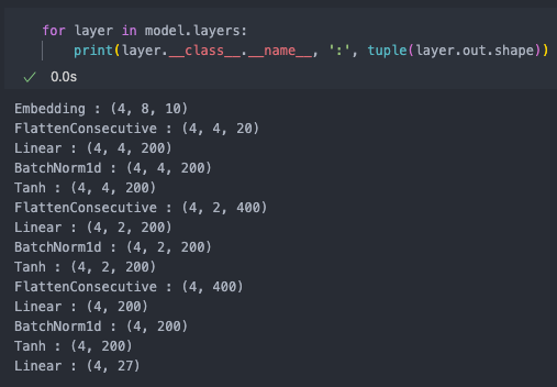
Basically, every time we go through a FlattenConsecutive(2), we reduce the number of groups by 2. In the last FlattenConsecutive, since we end up with a single group, that dimension gets squeezed out. Doing FlattenConsecutive(2) 3 times is equivalent (in terms of shape) of calling FlattenConsecutive(8) a single time.

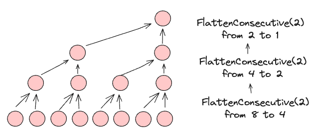
Also note that every time we go through a Linear layer, we fan-out back to 200 channels. This does not change. It is only the group dimension that is being crushed at each FlattenConsecutive layer.

Reducing n_hidden

Before we move on, we will just reduce our n_hidden (or channel dimension) from 200 to 68 so that our total number of parameters stays approximately the same.

This will allow our performances to be more comparable, and allow us to isolate the impact of progressive fusing, and not conflating that with just increasing the number of parameters.

The performance ends up being about the same as before.

Fixing BatchNorm1d

So recall our implementation of batch norm. The key thing that is happening here is that we are calculating the mean and variance over the entire batch. However, now that we have introduced more batch dimensions, we are instead calculating the mean and variance for each group independently. This is not what we want.

class BatchNorm1d:
  def __call__(self, x):
    # calculate the forward pass
    if self.training:
      xmean = x.mean(dim, keepdim=True) # batch mean
      xvar = x.var(dim, keepdim=True) # batch variance
    else:
      xmean = self.running_mean
      xvar = self.running_var
    xhat = (x - xmean) / torch.sqrt(xvar + self.eps) # normalize to unit variance
    self.out = self.gamma * xhat + self.beta
    # update the buffers
    if self.training:
      with torch.no_grad():
        self.running_mean = (1 - self.momentum) * self.running_mean + self.momentum * xmean
        self.running_var = (1 - self.momentum) * self.running_var + self.momentum * xvar
    return self.out

To fix this, we need to make sure we mean over this extra dimension if it exists. Just note that our implementation here deviates from PyTorch’s implementation of BatchNorm1d. We always expect the channel dimension to be the last dimension, whereas in PyTorch they always expect channel dimension to be the 1st dimension.

class BatchNorm1d:
  def __call__(self, x):
    # calculate the forward pass
    if self.training:
      if x.ndim == 2:
        dim = 0
      elif x.ndim == 3:
        dim = (0,1)
      xmean = x.mean(dim, keepdim=True) # batch mean
      xvar = x.var(dim, keepdim=True) # batch variance
    else:
      xmean = self.running_mean
      xvar = self.running_var
    xhat = (x - xmean) / torch.sqrt(xvar + self.eps) # normalize to unit variance
    self.out = self.gamma * xhat + self.beta
    # update the buffers
    if self.training:
      with torch.no_grad():
        self.running_mean = (1 - self.momentum) * self.running_mean + self.momentum * xmean
        self.running_var = (1 - self.momentum) * self.running_var + self.momentum * xvar
    return self.out

With this fix, we performance improves just a bit.

Scaling up

With this new architecture, we can easily scale up our model. Let’s increase n_embd from 10 to 24 and n_hidden from 68 to 128.

# final hierarchical network
n_embd = 24 # the dimensionality of the character embedding vectors
n_hidden = 128 # the number of neurons in the hidden layer of the MLP
model = Sequential([
  Embedding(vocab_size, n_embd),
  FlattenConsecutive(2), Linear(n_embd * 2, n_hidden, bias=False), BatchNorm1d(n_hidden), Tanh(),
  FlattenConsecutive(2), Linear(n_hidden*2, n_hidden, bias=False), BatchNorm1d(n_hidden), Tanh(),
  FlattenConsecutive(2), Linear(n_hidden*2, n_hidden, bias=False), BatchNorm1d(n_hidden), Tanh(),
  Linear(n_hidden, vocab_size),
])

Performance gets a bit better but since we don’t have an experimental harness its going to be hard for us to tune these numbers any further.

Convolution is like a for-loop

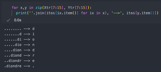
Let’s say we are only considering this one name, which gives us 8 independent examples.

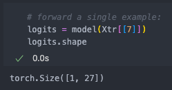
If we wanted to forward this single example, we can put the single example in a 1D tensor.

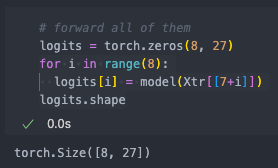
If we wanted to forward all 8 examples, we could put it in a for loop but we would then have to call our model 8 times (one for each example).

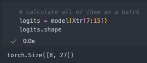
We could also calculate all of them at the same time as a batch, but we are still treating each of the examples as independent examples.

If we consider the original diagram in the Wavenet paper, what we implemented is basically just the black tree-like structure which calculates a single output. Even if we batched all of our 8 examples, we would need to then recreate the tree 8 times, each one unit shifted over. With convolutions (which we did not implement), the intermediate nodes actually can get reused since we are computing all of the outputs in parallel (ie the dotted lines).